Page 323 - IJB-8-4

Bonatti, et al.
A

B C

D E

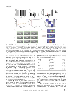
Figure 4. (A) The validation accuracy and loss for the selection experiments (presented as a mean across the 5-fold of the cross-validation
procedure), as well as the number of parameters for each tested model. (B) The training loss and accuracy curves for the selected model
(depth = 6 and a simple “conv block”). The dashed lines represent the original data points, while the solid lines are the results of a moving
average filter (window size of 3) for better visualization. The red vertical dashed lines represent the epoch at which the model was saved
during early stopping (epoch = 6). (C) The confusion matrix obtained by classifying the dataset using the model trained in (b). (D and E)
The results of the classification invariance to zoom and focus and the grad-CAM activations on three example prints, respectively. The green
border in (D) represents a correct prediction by the model (all images refer to an “ok” print).
models (in terms of depth and “conv block” type) reached Table 4. Summary of the overall and per-class metrics computed
high mean accuracies (above 90%) on the 5-fold of the from the confusion matrix on the test set
cross-validation procedure. The results from the two-way Group Metric Value
ANOVA tests showed no statistically significant effects of Overall Accuracy 94.3%
the two tested parameters on both the validation accuracy “ok” Precision 87.2%
and loss (P > 0.05 for both cases). As a result, we chose Recall 96.5%
the final model based on the number of parameters (which “over_e” Precision 98.3%
is an indication of the model complexity). Considering Recall 94.5%
the graph in Figure 4A, we selected the configuration
with depth = 6 and a simple “conv block,” representing “under_e” Precision 97.6%
an intermediate solution between a high (meaning slower Recall 92.2%
computation time) and low complexity (which may not
generalize well to new printing scenarios). The optimized dataset, the actual shape of the scaffold for each class did
DL model showed a fast computing time of around 182 not show a great variability, making the problem easy to
ms to classify 30 frames (average of 10 runs on CPU), learn for the model. The confusion matrix in Figure 4C,
which is compatible with the 1 s sampling frequency for computed using the saved model at this step, shows
the in-process monitoring application. that the DL model can predict correctly over the dataset
Figure 4B reports the training loss and accuracy with high values of the computed metrics, as reported in
curves for the final model. The model started over-fitting Table 4.
after just 6 epochs, as confirmed by the increase of the It is important to note that for the “ok” class the
test loss curve. This may be due to the fact that, even if precision is significantly lower than the precision for
a set of augmentation operations had been applied to the the other classes. This means that the DL model may

International Journal of Bioprinting (2022)–Volume 8, Issue 4 315