Page 98 - IJB-9-2

International Journal of Bioprinting Holistic charge-based MEW scaffold model

3. Results and discussion to calculate the electric potential difference between two
arbitrary points P and O around an infinitely long uniform
3.1. Model development charge line, which is as follows.
As stated before, the analytical model proposed herein
comprehensively considers all of the charges in all of the ϕ P () − () = 2 k λ ln r O (I)
ϕ O
fibers in the topmost two layers of the scaffold, so it is a 0 r P
more complicated but more panoramic approximation of
the actual process. To establish the holistic model, several ϕ(P) and ϕ(O) are the electric potential at point P
simplifying assumptions are formulated, as schematized in and O, respectively. k is the Coulomb constant and λ
0
Figure 2. First, the charges (both positive and negative) in is the linear charge density. r and r are the distances
o
p
both the incoming jet segment of interest and the deposited from point P and O to the charge line, respectively. If
fibers are polarized by the external electric field. Since the O is selected as the zero point of potential energy, then
incoming jet segment of interest (Figure 2A blue slice) is ϕ(O) = 0.
approximately oriented parallel with respect to the Y-axis If P is occupied by the charge segment and O is
at the time instant, as shown in Figure 2A, the charges in occupied by the origin of the coordinates system, as shown
it can be modeled as a pair of charge segments (Figure 2B in Figure 2A–C, the contribution of charge line ③ in
red and black points), and all of the positive or negative Fiber A to the electric potential energy of charge segment
charges are located at the corresponding equivalent charge ① in the incoming jet segment in Figure 2C is:
centroids. The charge segment herein is referred to as
a charge line with an infinitesimally small length. While 2 2
for the already deposited fibers, the entrapped polarized E = k q dl ln   (0.5 1 S  + ) f  + L (II)
2
charges are modeled as a pair of infinitely long uniform p(①→③) 0  X + (0.5 1 S  + ) 2 + Z 2
charge lines. In this way, all the charges within the  f 
topmost two layers of the scaffold can be modeled as two
charge grids (Figure 2B red and black grids). Second, as q is the negative charge density for both the charge
a panoramic consideration, the jet deposition accuracy is segment and charge line. dl is the line element of the
affected by all of the charges in the topmost two layers of incoming jet segment of interest. d is the fiber diameter.
f
the scaffold. However, deposited fibers in more previous S is the interfiber distance according to the prescribed
f
layers are not considered herein. Finally, the excess toolpath. L is half of the distance between the centroids
material accumulation at the intersecting points is not for the positive and negative charges. X and Z are the
considered in this investigation. Possible problems caused coordinates of the incoming jet segment of interest.
by these assumptions and solutions to them are described Considering all the combinations of charge segments
in section 3.2.4. and charge lines, four terms will arise in the calculation

Based on the aforementioned assumptions, the model of the total electric potential energy related to Fiber A in
construction starts with a well-established formula used Figure 2B.

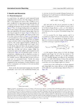
A B C

Figure 2. Schematic of jet deposition process. (A) Schematic of the incoming jet segment of interest (in blue) approaching the topmost two layers of the
scaffold. (B) The incoming jet segment of interest is modeled as a pair of charge segments whose charge amount are qdl and Qdl, respectively. Each fiber
in the topmost two layers of the scaffold is modeled as two infinitely long uniform charge lines, whose linear charge densities are q and Q , respectively. In
0
this way, all positive (negative) charge lines in the topmost two layers form a positive (negative) charge grid. The grey plane in (A) denotes the midplane
between the positive and negative charge grids, whose center defines the origin of the coordinates system. (C) is the side view of (A) and (B) with polymer
material and charge superimposed together. The distance between the centroids of positive and negative charges is 2L. The interfiber distance is S . The fiber
f
diameter is d. Fiber A is an arbitrary deposited fiber in the topmost two layers of the scaffold. ① (or ②) and ③ (or ④) denote the positive (or negative)
f
charge segment in the incoming jet segment of interest and charge line in Fiber A, respectively.
Volume 9 Issue 2 (2022) 90 https://doi.org/10.18063/ijb.v9i2.656