Page 131 - IJOCTA-15-4

Fixed-time sliding mode control with disturbance observer and variable exponent coefficient for nonlinear
systems
Remark 1. Unlike global fixed-time sta-
bility, practical fixed-time stability implies con-
vergence of tracking errors to a specific re-
gion around the origin rather than to the ex-
act origin. This concept is often more applica-
ble to real-world scenarios, such as motors and
robotic manipulator systems, 42,43 especially in
controllers employing DOs or adaptive approxi-
mators.
To better understand system stability, we re-
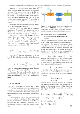
fer to the following key lemmas: Figure 1. Block diagram of the control architecture
Lemma 1. 22,44 Let V (y) be a Lyapunov Abbreviations: FTTSMC, fixed-time trajectory
tracking sliding mode control; FVECDO, fixed-time
function for System IV with parameters α, β ∈
+
+
ℜ , 0 < q 1 < 1, q 2 > 1, and υ ι ∈ ℜ , sat- variable exponent coefficient disturbance observer.
˙
isfying the inequality V (y) ≤ −αV (y) q 1 −
βV (y) q 2 + υ ι . Then, the system is prac- 3.1. Fixed-time variable exponent
coefficient disturbance observer
tically fixed-time stable, and the residual
design
set is defined as: R ι = {y|V (y) ≤ min
n oo
(υ ι / ((1 − υ θ ) β) ) 1/q 2 , (υ ι / ((1 − υ θ ) α) ) 1/q 1 Lumped disturbances can adversely affect the tra-
jectory tracking performance of nonlinear dynam-
where 0 < υ θ < 1, and the time bound for con-
ical systems. To improve performance, these
vergence is given in Equation (5):
lumped disturbances must be estimated and com-
pensated for as early as possible. Therefore, this
1 1 section introduces the FVECDO for accurate es-
n
T (y 0 ) ≤ + , ∀y 0 ∈ ℜ . (5) timation of lumped disturbances, starting with a
α (1 − q 1 ) β (q 2 − 1)
reformulation of the error model as follows:
Lemma 2. 45 For any constants ς > 0 and ˙ ∗
l ∈ ℜ, the following inequality holds Equation ∗ Ξ 2 = −ℓ 1 Ξ 2 + h (x) u + d (7)
(6): where d = G (x)+ℓ 1 Ξ 2 +D a and ℓ 1 denote a real
positive constant. According to Equation (7), an
˙
ˆ
auxiliary state Ξ 2 is introduced to define an aux-
|l|

0 ≤ |l| − |l| tanh ≤ ϖς (6) iliary system as in Equation (8):
ς
˙
ˆ
ˆ
where ϖ denotes a constant that meets the con- Ξ 2 = −ℓ 1 Ξ 2 + h (x) u (8)
ˆ
dition ϖ = e −ϖ−1 , e.g ϖ = 0.2785. Let Θ 1 = Ξ 2 − Ξ 2 denote the error between
ˆ
Notation: For any real number y, the ex- the Ξ 2 and Ξ 2 . Substituting Equations (7) and
a
a
pression sig(y) = |y| sign (y) , with sign (.) de- (8) into the derivative of Θ 1 yields the following
notes the sign function, and a is a positive con- dynamics:
stant.
˙
Θ 1 = −ℓ 1 Θ 1 + d ∗
(9)
Θ 2 = ℓ 2 Θ 1
∗
where ℓ 2 is a real positive constant, d represents
3. Main results
the unknown system input, and Θ 2 can be re-
This paper presents the design of a novel garded as the system output. Using Equations
FTTSMC using FVECDO estimation for System (7)–(9), the FVECDO is formulated as in Equa-
I, aiming to ensure that the system states reach tion (10):
a small neighborhood of the origin within a pre-
˜
determined finite time, regardless of initial condi- ˆ ˆ −1 ˙ ˜ ϕ(Θ 1) ˜
˙
tions. Θ 1 = −ℓ 2 ℓ 3 Θ 1 + ℓ 2 Θ 2 + α 1 χ Θ 1 sign Θ 1
Furthermore, the controller parameters al- ˜ ˜ Υ
+ ℓ 3 Θ 2 + α 2 Θ 1 + α 3 sig Θ 1
lowed for effective adjustment of the upper limit

on the settling time. Figure 1 illustrates the d = ℓ −1 ℓ 1 ℓ 2 Θ 1 + Θ 2
ˆ ∗
˙
ˆ
structure of the closed-loop trajectory track- 2
ˆ
ˆ ∗
ing system resulting from this control strat- D a = d − ℓ 1 Ξ 2 − G (x)
egy. (10)
673