Page 135 - IJOCTA-15-4

Fixed-time sliding mode control with disturbance observer and variable exponent coefficient for nonlinear
systems
It can be observed that the form of Equation 4.1. Example 1
(37) is the same as that of Equation (12), and the 14
Consider the SIP from Zuo as an example. Its
convergence area of the sliding variable is deter-
dynamics can be expressed in the same form as
mined as shown in Equation (38):
Equation (1), with g (x) , h (x), and D a defined
as follows:
s
2

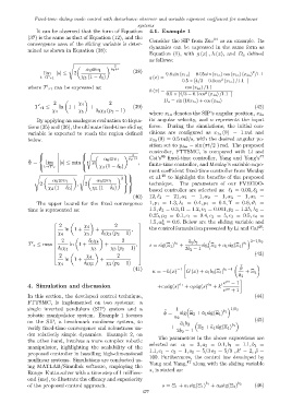
α 6 ϖυ 1 p 2 +1
lim |s| ≤ 2 (38) 9.8 sin (x 1a ) − 0.05 sin (x 1a ) cos (x 1a ) (x 2a ) /1.1
2
′ χ 3 (1 − δ 0 )
t→T r1 g (x) =
2
0.5 × [4/3 − 0.1cos (x 1a ) /1.1 ]
′
where T r1 can be expressed as: cos (x 1a ) /1.1
h (x) =
2
0.5 × [4/3 − 0.1cos (x 1a ) /1.1 ]
D a = sin (10x 1a ) + cos (x 2a )
2 χ 4 2
′
T r1 ≤ ln 1 + + (39) (42)
χ 4 χ 5 δ 0 χ 3 (p 2 − 1)
where x 1a denotes the SIP’s angular position, x 2a
By applying an analogous evaluation to Equa- its angular velocity, and u represents the input
tions (35) and (36), the ultimate fixed-time sliding force. During the simulations, the initial con-
variable is expected to reach the region defined ditions are configured as x 1a (0) = 1 rad and
below. x 2a (0) = 0.5 rad/s, with the desired angular po-
sition set to y des = sin (πt/2 ) rad. The proposed
controller, FTTSMC, is compared with Li and
 s
2
46 47
  p 2 +1 Cai’s fixed-time controller, Yang and Yang’s
α 6 ϖυ 1
Φ = lim |s| ≤ min 2 , finite-time controller, and Moulay’s variable expo-
′ χ 3 (1 − δ 0 )

nent coefficient fixed-time controller from Moulay
t→T r

s
s 48
et al. to highlight the benefits of the proposed
2
α 6 ϖυ 1 α 6 ϖυ 1
2 , 2 technique. The parameters of our FVECDO-
χ 4 (1 − δ 0 ) χ 5 (1 − δ 0 )
based controller are selected as: ℓ 1 = 0.03, ℓ 2 =

(40) 12, ℓ 3 = 21, α 1 = 1, α 2 = 1, α 3 = 1, α 5 =
The upper bound for the fixed convergence 1, p 1 = 1.3, λ 1 = 0.4, µ 1 = 0.1, Υ = 0.6, ϑ 1 =
time is represented as: 1.5, ϑ 2 = 0.3, Ω = 1.2, υ 1 = 0.001, p 2 = 1.25, λ 2 =
0.25, µ 2 = 0.1, c 1 = 0.4, c 2 = 5, c 3 = 0.5, c 4 =
∗
1.5, α = 0.6. Below are the sliding variable and

2 χ 4 2 46
  6
ln 1 + + , the control formulation presented by Li and Cai :
χ 4 χ 5
 δ 0 χ 3 (p 2 − 1) 
 


′  2 δ 0 χ 4 2  b 1 ¯ a 2 b 2 b 1 2−1/b 2
T r ≤ max  ln 1 + + ,  s = sig(Ξ 1 ) + sig Ξ 2 + ¯a 1 sig(Ξ 1 )
δ 0 χ 4 χ 5 χ 3 (p 2 − 1)  2b 2 − 1
 
(43)
2 2
 χ 4 
ln 1 + +
χ 4 δ 0 χ 5 χ 3 (p 2 − 1)
¯
(41) −1 b 1 −1 ϕ
u = −h(x) G (x) + ¯a 1 b 1 |Ξ 1 | + Ξ 2
¯ a 1

4. Simulation and discussion +c 1 sig(s) o 1 + c 2 sig(s) o 2 + k ′ e ¯ ρs − 1
e ¯ ρs + 1
In this section, the developed control technique, (44)
FTTSMC, is implemented on two systems: a
single inverted pendulum (SIP) system and a ¯ 1 b 1 1/b 2
robotic manipulator system. Example 1 focuses ϕ = ¯ a 2 sig Ξ 2 + ¯a 1 sig(Ξ 1 )
on the SIP, a benchmark nonlinear system, to ¯ a 1 b 2 (45)
verify fixed-time convergence and robustness un- + 2b 2 − 1 Ξ 2 + ¯a 1 sig(Ξ 1 ) b 1
der relatively simple dynamics. Example 2, on
the other hand, involves a more complex robotic The parameters in the above expressions are
manipulator, highlighting the scalability of the selected as: ¯a 1 = 3, ¯a 2 = 0.1, b 1 = 1.1, b 2 =
′
1.1, c 1 = c 2 = 1, o 1 = 5/3 o 2 = 5/9 , k = 2, ¯ρ =
proposed controller in handling high-dimensional
100. Furthermore, the control law developed by
nonlinear systems. Simulations are conducted us-
Yang and Yang, 47 along with the sliding variable
ing MATLAB/Simulink software, employing the
s, is stated as:
Runge–Kutta solver with a time step of 1 millisec-
ond (ms), to illustrate the efficacy and superiority
b 1
of the proposed control approach. s = Ξ 1 + ¯a 1 sig(Ξ 1 ) + ¯a 2 sig(Ξ 2 ) b 2 (46)
677