Page 138 - IJOCTA-15-4

Anjum et al. / IJOCTA, Vol.15, No.4, pp.670-685 (2025)
′
′
′
−∆Z ι (x)x 2a − ∆G ι (x 1a ) The disturbance term in 2, β = 5/3 , ξ = 2, b 1 = b 2 = 1,k = 2, λ 0 =
the model is expressed as given in Equation (50): λ 1 = λ 2 = 1. The initial conditions for the
joint positions are selected as q ι1 (0) = 1rad, and
" #
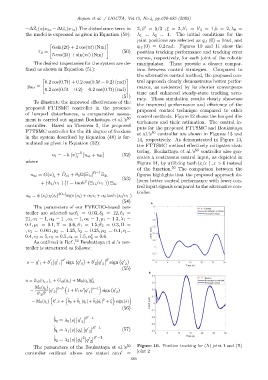
6 sin(2t) + 2 cos(πt) (Nm) q ι2 (0) = 0.2 rad. Figures 10 and 11 show the
τ d = (50) position tracking performance and tracking error
5 cos(2t) + sin(πt) (Nm)
curves, respectively, for each joint of the robotic
The desired trajectories for the system are de- manipulator. These provide a clearer compar-
fined as shown in Equation (51): ison between control strategies. Compared to
the alternative control method, the proposed con-
" #
0.2 cos(0.7t) + 0.2 cos(0.5t − 0.2) (rad) trol approach clearly demonstrates better perfor-
y des = mance, as evidenced by its shorter convergence
0.2 cos(0.5t − 0.2) − 0.2 cos(0.7t) (rad)
time and enhanced steady-state tracking accu-
(51)
racy. These simulation results clearly showcase
To illustrate the improved effectiveness of the the improved performance and efficiency of the
proposed FTTSMC controller in the presence
proposed control technique compared to other
of lumped disturbances, a comparative assess- control methods. Figure 12 shows the lumped dis-
ment is carried out against Boukattaya et al.’s 50
turbances and their estimation. The control in-
controller. Based on Theorem 2, the proposed
puts for the proposed FTTSMC and Boukattaya
FTTSMC controller for the ith degree of freedom 50
et al.’s controller are shown in Figures 13 and
in the system described by Equation (48) is for-
14, respectively. As demonstrated in Figure 13,
mulated as given in Equation (52):
the FTTSMC method effectively mitigates chat-
tering. Boukattaya et al.’s 50 controller also gen-
−1
u i = −h (x) [u ai + u bi ] (52)
i erates a continuous control input, as depicted in
where Figure 14, by utilizing tanh (x/ε ) , ε > 0 instead
of the function. 50 The comparison between the
ˆ
u ai = G(x) + D ai + ϑ 1 Ω|Ξ 1i | Ω−1 Ξ 2i figures highlights that the proposed approach de-
i (53)
2 livers better control performance with lower con-
+ (ϑ 2 /υ 1 ) 1 − tanh (Ξ 1i /υ 1 ) Ξ 2i
trol input signals compared to the alternative con-
troller.
ϕ(s i )
u bi = ψ (s i ) χ(s i ) sign (s i ) + α 5 s i + α 6 tanh (s i /υ 1 )
(54)
The parameters of our FVECDO-based con-
troller are selected as:ℓ 1 = 0.03, ℓ 2 = 12, ℓ 3 =
21, α 1 = 1, α 2 = 1 , α 3 = 1, α 5 = 1, p 1 = 1.3, λ 1 =
0.4, µ 1 = 0.1, Υ = 0.6, ϑ 1 = 1.5,ϑ 2 = 0.3, Ω =
, υ 1 = 0.001, p 2 = 1.25, λ 2 = 0.25, µ 2 = 0.1, c 1 =
∗
0.4, c 2 = 5, c 3 = 0.5, c 4 = 1.5, α = 0.6.
6
As outlined in Ref., 50 Boukattaya et al.’s con-
troller is structured as follows:

β
α
′

s = q + b 1 q 1 ′ sign q ′ 1 + b 2 q 2 ′ sign q ′ 2
′ ′
1
′ ′
(55)
u = Z ι0 (q , ι ) ι + G ι0 (q ) + M 0 (q )¨y ′ d
ι
ι
ι
M 0 (q ) 2−β ′ α−1 ′
− ι ′ 1 + b 1 α q 1 sign q 2
q
′ ′
2
′
b 2 β ′
2
ˆ
ˆ
′
ˆ
− M 0 (q ) k .s + b 0 + b 1 |q ι | + b 2 | ˙q ι | + ξ sign(s)
ι
(56)
˙
β −1
ˆ ′ ′
b 0 = λ 0 |s| q
2
˙
β −1
ˆ ′ ′ (57)
b 1 = λ 1 |s| |q ι | q
2
˙
β −1
ˆ 2 ′ ′
b 2 = λ 2 |s| | ˙q ι | q
2
The parameters of the Boukattaya et al.’s 50 Figure 10. Position tracking for (A) joint 1 and (B)
controller outlined above are stated as:α ′ = joint 2
680