Page 136 - IJOCTA-15-4

Anjum et al. / IJOCTA, Vol.15, No.4, pp.670-685 (2025)

−1 1 b 1 −1 2−b 2
u = −h(x) G (x) − sig Ξ 2 1 + ¯a 1 b 1 |Ξ 1 |
¯ a 2 b 2
+c 1 sig(s) o 1 + c 2 sig(s) o 2 + k ′ e ¯ ρs − 1
e ¯ ρs + 1
(47)

The parameters in the above expressions are
selected as follows: ¯ a 1 = 5, ¯a 2 = 0.1, b 1 =
′
1.1, b 2 = 1.1, c 1 = c 2 = 1, o 1 = 5/3 ,o 2 = 5/9, k =
2, ¯ρ = 100. The parameters for Moulay’s variable
exponent coefficient fixed-time controller are set
as in Moulay et al. 48 The angular position track-
ing of the SIP and the angular position tracking
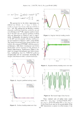
error are illustrated in Figures 2 and 3, respec- Figure 4. Angular velocity tracking results
tively. Additionally, the angular velocity tracking
of the SIP and the angular velocity tracking er-
ror are depicted in Figures 4 and 5, respectively.
The figures demonstrate that among the four con-
trollers, the proposed FTTSMC exhibits superior
performance, with faster convergence and better
steady-state control accuracy in the presence of
lumped disturbances. Furthermore, Figure 6 dis-
plays the lumped disturbances and their estima-
tion, highlighting that the FVECDO performs
exceptionally well by accurately estimating the
lumped disturbances within a fixed-timeframe.

Figure 5. Angular velocity tracking error over time

Figure 2. Angular position tracking results

Figure 6. Estimated lumped disturbances

Three distinct sets of initial state condi-
tions IV1 = [x 1a , x 2a ] = [1 rad, 0.5 rad/s] , IV2 =
[x 1a , x 2a ] = [3 rad, 0.0 rad/s] ,IV3 = [x 1a , x 2a ] =
[5 rad, 1 rad/s] are used in the second phase of the
Figure 3. Position tracking errors over time
SIP simulations to assess the effectiveness of the
678