Page 137 - IJOCTA-15-4

Fixed-time sliding mode control with disturbance observer and variable exponent coefficient for nonlinear
systems
proposed control approach under external distur- the actuator inputs applied to the system. The
bances and model uncertainties. The parameters matrix Z ι (q ι , ˙q ι ) ∈ R n×n accounts for centripetal
n
of the FTTSMC scheme are tuned based on the and Coriolis forces. G ι (q ) ∈ ℜ represents the
ι
n
earlier analysis. Tracking errors for angular po- gravity vector, and τ d ∈ ℜ indicates the exter-
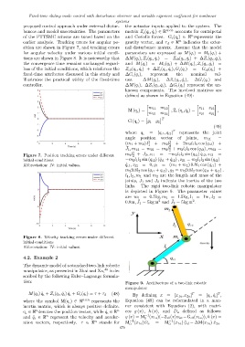
sition are shown in Figure 7, and tracking errors nal disturbance matrix. Assume that the model
for angular velocity under various initial condi- parameters are expressed as M(q ι ) = M 0 (q ι ) +
tions are shown in Figure 8. It is noteworthy that ∆M(q ι ), Z ι (q ι , ˙q ι ) = Z ι0 (q ι , ˙q ι ) + ∆Z ι (q ι , ˙q ι ),
the convergence time remains unchanged regard- and M(q ι ) = M 0 (q ι ) + ∆M(q ι ), Z ι (q ι , ˙q ι ) =
less of the initial conditions, which reinforces the Z ι0 (q ι , ˙q ι ) + ∆Z ι (q ι , ˙q ι ), G ι (q ι ) = G ι0 (q ι ) +
fixed-time attributes discussed in this study and ∆G ι (q ι ), represent the nominal val-
illustrates the practical utility of the fixed-time ues. ∆M(q ι ), ∆Z ι (q ι , ˙q ι ), ∆G ι (q ι ) and
controller. ∆M(q ι ), ∆Z ι (q ι , ˙q ι ), ∆G ι (q ι ) represent the un-
known components. The involved matrices are
defined as shown in Equation (49):

m 11 m 12 z 11 z 12
M (q ) = , Z ι (q ,˙q ) = ,
ι
ι
ι
m 21 m 22 z 21 z 22
T

G (q ) = g 1 g 2
ι
(49)
where q ι = [q ι1 , q ι2 ] T represents the joint
angle position vector of joints, m 11 =
(m 1 + m 2 ) l 2 + m 2 l 2 2 + 2m 2 l 1 l 2 cos (q ι2 ) +
1
¯
2
J 1 , m 12 = m 21 = m 2 l + m 2 l 1 l 2 cos (q ι2 ) , m 22 =
2
2 ¯ = =
Figure 7. Position tracking errors under different m 2 l + J 2 , z 11 −m 2 l 1 l 2 sin (q ι2 ) ˙q ι2 , z 12
2
initial conditions −m 2 l 1 l 2 sin (q ι2 ) ( ˙q ι1 + ˙q ι2 ) , z 21 = m 2 l 1 l 2 sin (q ι2 )
Abbreviation: IV: initial values. ˙ q ι1 , z 22 = 0, g 1 = (m 1 + m 2 ) 9.8l 1 cos (q ι1 ) +
m 2 9.8l 2 cos (q ι1 + q ι2 ) , g 2 = m 2 9.8l 2 cos (q ι1 + q ι2 ) .
l 1 , l 2 , m 1 and m 2 are the length and mass of the
¯
¯
joints, J 1 and J 2 indicate the inertia of the two
links. The rigid two-link robotic manipulator
is depicted in Figure 9. The parameter values
are m 1 = 0.5kg, m 2 = 1.5kg, l 1 = 1m, l 2 =
¯
¯
2
2
0.8m, J 1 = 5kg m and J 2 = 5kg m .
Figure 8. Velocity tracking errors under different
initial conditions
Abbreviation: IV: initial values.

4.2. Example 2
The dynamic model of a standard two-link robotic
manipulator, as presented in Zhai and Xu, 49 is de-
scribed by the following Euler–Lagrange formula-
tion: Figure 9. Architecture of a two-link robotic
manipulator
T
M(q ι ) ¨q ι + Z ι (q ι , ˙q ι ) ˙q ι + G ι (q ι ) = τ + τ d (48) By defining x = [x 1a , x 2a ] T = [q ι , ˙q ι ] ,
where the symbol M(q ) ∈ ℜ n×n represents the Equation (48) can be reformulated in a man-
ι
inertia matrix, which is always positive definite. ner consistent with Equation (2), with matri-
n n
q ∈ ℜ denotes the position vector, while ˙q ι ∈ R ces g (x) , h (x), and D a defined as follows:
ι
n
and ¨q ι ∈ R represent the velocity and acceler- g (x) = M −1 (x 1a )(−Z ι0 (x)x 2a −G ι0 (x 1a )), h (x) =
0
ation vectors, respectively. τ ∈ ℜ n stands for M −1 (x 1a )D a = M −1 (x 1a ) (l d − ∆M(x 1a ) ˙x 2a
0 0
679