Page 189 - IJOCTA-15-4

Proportional integral derivative plus control for nonlinear discrete-time state-dependent parameter. . .
By substituting Equation (19) into Equation (18), By substituting T (t) nn from Equation(28) and
one obtains ∆ξ from Equation (27) into Equation (26), one
T
T
˜
˙
V (e, ϑ, ˜υ) = −e (Q)e + 2e PB∆ξ (20) gets
Since P is a matrix that is symmetric +ve defi- T ∗T
ˆT
ϑ x + ˆυ r + W h(e) + ε
nite and A p is Hurwitz; thus, we get the Lyapunov ˙ x = Ax + B ˆ T .
T
equation PA p + A P = −Q and Q > 0 is also a −W h(e) − Ke
p
+ve definite symmetric matrix. (29)
Equation (29) can be written as
To find the asymptotic stability of the MRAC-
h i
˜ T
ˆ T
T
TDE approach, one can get the following equa- ˙ x = Ax + B ϑ x + ˆυ r − W h(e) + ε − Ke .
tion:
(30)
˙
˜
T
T
V (e, ϑ, ˜υ) = −e (Q)e + 2e PB∆ξ where W = W − W ∗T .
˜ T
ˆ T
2
≤ −λ m (Q)∥e∥ + 2 ∥e∥ ∥PB∥ ∥∆ξ∥ . (21) The tracking error dynamics ˙e = ˙x − ˙x p using
Equations (9) and (30) is defined as
2 ∥PB∥ ∥∆ξ∥
∥e∥ ≤ . (22) h i T
ˆT
˜ T
λ m (Q) ˙ e = A + Bϑ x + Bˆυ r − BW h(e) − BKe
˜
˙
⇒ V (e, ϑ, ˜υ) < 0. +Bε − A p x p − B p r ± A p x.
Hence, the closed MRAC-TDE system is asymp- (31)
totically stable. When one solves Equation (31), it yields
T
˜ T
˜ T
˙ e = A p e+Bϑ x+B˜υ r−BW h(e)−BKe+Bε.
(32)
˜
ˆ
3.2. MRAC-NNTDE control design where ϑ = ϑ − ϑ and ˜υ = ˆυ − υ are the adaptive
errors, and the ϑ and υ are the unknown gains.
In this section, MRAC-TDE with a neural net-
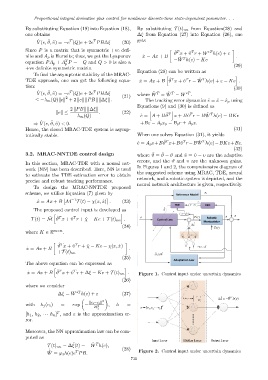
In Figures 1 and 2, the comprehensive diagram of
work (NN) has been described. Here, NN is used
the suggested scheme using MRAC, TDE, neural
to estimate the TDE estimation error to obtain
network, and a robotic system is depicted, and the
precise and robust tracking performance.
neural network architecture is given, respectively.
To design the MRAC-NNTDE proposed
scheme, we utilize Equation (7) given by
¯ −1

˙ x = Ax + B M T (t) − χ(x, ˙x) . (23)
The proposed control input is developed as
h i
T
¯ ˆ T
T (t) = M ϑ x + ˆυ r + ˆχ − Ke + T (t) nn .
(24)
where K ∈ ℜ m×n .
T
ˆT
ϑ x + ˆυ r + ˆχ − Ke − χ(x, ˙x)
˙ x = Ax + B .
+T (t) nn
(25)
The above equation can be expressed as
h i
T
ˆ T
˙ x = Ax + B ϑ x + ˆυ r + ∆ξ − Ke + T (t) nn . Figure 1. Control input under uncertain dynamics
(26)
where we consider
∆ξ = W ∗T h(e) + ε (27)

∥e i −c j ∥ 2
with h j (e i ) = exp − , h =
2b 2
j
T
[h 1 , h 2 , · · · h n ] , and ε is the approximation er-
ror.
Moreover, the NN approximation law can be com-
puted as
ˆ
ˆ T
T (t) nn = ∆ξ(t) = −W h(e), (28)
˙
ˆ
T
W = φ 3 h(e)e PB. Figure 2. Control input under uncertain dynamics
731