Page 66 - IJPS-11-1

International Journal of
Population Studies Macroeconomic factors and housing dynamics

Appendix

Solution algorithm
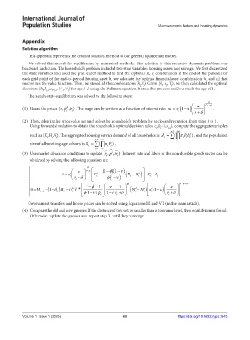
This appendix represents the detailed solution method to our general equilibrium model.
We solved this model for equilibrium by numerical methods. The solution to this recursive dynamic problem was
backward induction. The household’s problem included two state variables: housing assets and savings. We first discretized
the state variables and used the grid search method to find the optimal (h, s) combination at the end of the period. For
each grid point of the end-of-period housing asset h , we calculate the optimal financial asset combination {h and s } that
J
J
J
maximizes the value function. Then, we stored all the combinations (h S ). Given {h , s , V }, we then calculated the optimal
J, J
J
J
J
decisions {h ,h ,s ,s ,V ,V } for age J−1 using the Bellman equation. Iterate this process until we reach the age of 1.
J-1 J J-1
J
J
J-1
The steady-state equilibrium was solved by the following steps:

1 ( )
c
(1) Guess the prices {,rp� t h ,}tr . The wage can be written as a function of interest rate: w 1 .
z

t
t
t
t
r
t
(2) Then, plug in the price value set and solve the household’s problem by backward recursion from time J to 1.
Using forward simulation to obtain the household’s optimal decision rules {c ,h +1,s }, compute the aggregate variables
t
t
t+1
= jJ = i j
π Ph
such as {K ,H,N}. The aggregated housing service demand of all households is H t = ∑∏ it j t j ) , and the population
(

t
t
t

jJr ij

t
size of all working-age cohorts is N ( it j = j 1 = i 1
P ) .
j1 i1

(3) Use market clearance conditions to update {,rp h t
,}tr . Interest rate and labor in the non-durable goods sector can be
t
obtained by solving the following equation set:
 1 α  α
 0 z  = c  α  − N −  c (1 φ − )(1 α − ) N c  C − I
 t  r + δ    t φ (1 ν − ) ( N − t t ) −    t t

 t 
− +
  − 1   ν 1  φν   α   1 φ φν
h
0 H − (1 δ − )H − () 1 νφ  1 φ −    ( N − l N c ) z  c (1 α − )  
z
=
 t + 1 h t t  φ (1 ν − ) p l     1 ν − r + t δ  t t  t  r + t δ    

Government transfers and house prices can be solved using Equations III and VII (in the main article).
(4) Compare the old and new guesses. If the distance of two sets is smaller than a tolerance level, then equilibrium is found.
Otherwise, update the guesses and repeat step 3, until they converge.

Volume 11 Issue 1 (2025) 60 https://doi.org/10.36922/ijps.3645