Page 107 - IJPS-11-2

International Journal of
Population Studies Do female-headed households have poorer finances?

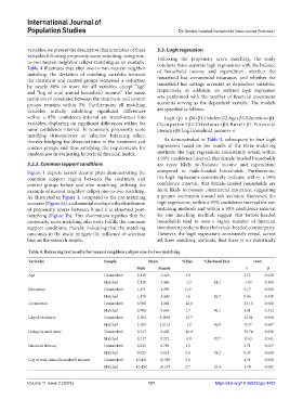
variables, we present the descriptive characteristics of these 3.3. Logit regression
variables following propensity score matching, using one- Following the propensity score matching, the study
to-two nearest neighbor caliper matching as an example. conducts three separate logit regressions with the balance
Table 4 illustrates that after one-to-two nearest neighbor of household income and expenditure, whether the
matching, the deviation of matching variables between household has commercial insurance, and whether the
the treatment and control groups witnessed a reduction
by nearly 80% or more for all variables except “age” household has savings accounts as dependent variables,
and “log of total annual household income.” The mean respectively. In addition, an ordered logit regression
deviation of covariates between the treatment and control was performed with the number of financial investment
groups remains within 5%. Furthermore, all matching accounts serving as the dependent variable. The models
variables initially exhibiting significant differences are specified as follows:
within a 95% confidence interval are transformed into Logit (p) = β0+β1.Gender+β2.Age+β3.Education+β4.
variables, displaying no significant differences within the Occupation+β5.Citystatus+β6.Rural+β7.Financial
same confidence interval. In summary, propensity score literacy+β8.Log Household income+ ϵ
matching demonstrates an effective balancing effect,
thereby bridging the characteristics of the treatment and As demonstrated in Table 5, subsequent to four logit
control groups and thus satisfying the requirements for regressions based on the results of the three matching
randomness in evaluating household financial health. methods, the logit regressions consistently reveal, within
a 99% confidence interval, that female-headed households
3.2.3. Common support conditions are more likely to balance income and expenditure

Figure 1 depicts kernel density plots demonstrating the compared to male-headed households. Furthermore,
common support region between the treatment and the logit regressions consistently indicate, within a 99%
control groups before and after matching, utilizing the confidence interval, that female-headed households are
example of nearest neighbor caliper one-to-two matching. more likely to possess commercial insurance, suggesting
As illustrated in Figure 1, compared to the pre-matching a greater inclination toward risk aversion. Moreover, the
scenario (Figure 1a), a substantial overlap in the distribution logit regressions, within a 95% confidence interval for two
of propensity scores between 0 and 1 is observed post- matching methods and within a 90% confidence interval
matching (Figure 1b). This observation signifies that the for one matching method, suggest that female-headed
propensity score matching effectively fulfills the common households tend to own a higher number of financial
support conditions, thereby indicating that the matching investment products than their male-headed counterparts.
outcomes in the study mitigate the influence of selection However, the logit regressions consistently reveal, across
bias on the research results. all three matching methods, that there is no statistically

Table 4. Balancing test results for nearest neighbor caliper one‑to‑two matching
Variables Sample Mean %Bias %Reduced bias t‑test
Male Female t p
Age Unmatched 2.438 2.418 3.0 2.33 0.020
Matched 2.438 2.449 −1.7 44.1 −1.02 0.308
Education Unmatched 1.471 1.395 11.9 9.17 0.000
Matched 1.470 1.460 1.6 86.7 0.96 0.339
Occupation Unmatched 0.700 1.041 −42.8 −33.15 0.000
Matched 0.700 0.686 1.7 96.1 1.01 0.312
City of residence Unmatched 2.103 2.3639 −29.7 −22.91 0.000
Matched 2.103 2.1114 −1.0 96.8 −0.57 0.567
Living in rural areas Unmatched 0.217 0.402 −40.9 −29.74 0.000
Matched 0.217 0.222 −0.9 97.7 −0.63 0.531
Financial literacy Unmatched 0.825 0.792 3.5 2.71 0.007
Matched 0.825 0.818 0.8 78.2 0.47 0.638
Log of total annual household income Unmatched 10.431 10.305 5.8 4.31 0.000
Matched 10.432 10.373 2.7 53.4 1.74 0.082

Volume 11 Issue 2 (2025) 101 https://doi.org/10.36922/ijps.4403