Page 103 - IJPS-11-3

International Journal of
Population Studies Male fertility in Uganda

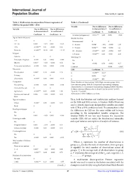
Table 3. Multivariate decomposition Poisson regression of Table 3. (Continued)
CEB for the period 2006 – 2016
Variable Due to differences Due to differences
Variable Due to differences Due to differences in characteristics E in coefficients C
in characteristics E in coefficients C Coefficient % Coefficient %
Coefficient % Coefficient % ≥2 wives (polygamous) −0.011*** 2.49 0.001 −0.14
Age at first birth (years) Marital duration
≤17 0 0 Never married 0 0
18 – 24 0.003 −0.71 0.001 −0.25 1 – 4 years 0.004* −0.91 −0.009 1.93
≥25+ −0.004*** 0.81 −0.001 0.16 5 – 9 years 0.002*** −0.48 −0.006 1.2
No birth −0.409*** 92.55 0.05 −11.37 10 – 14 years −0.020*** 4.63 −0.004 0.87
Religion ≥15 years −0.027*** 6.21 −0.01 2.16
Catholic 0 0 Watching TV
Protestant–Anglican −0.001 0.21 0.002 −0.49 No 0 0
Muslim 0.001* −0.25 −0.000 0.02 Yes −0.002 0.59 −0.001 0.17
Pentecostal and others −0.000 0.06 0.000 −0.02 Constant 0.046 −10.47
Education CEB Coefficient %
No education 0.000* 0.18 −0.001 17.3 E −0.498*** 112.7
Primary 0 0 C 0.056 −12.7
≥Secondary −0.005* 1.08 0.001 −0.18 R −0.442*** 100
Occupation Notes: Number of observations: 7,839; High-outcome group: 2016;
Not working −0.000 0.00 0.000 −0.04 Low-outcome group: 2006; E: Component representing changing
characteristics; C: Component representing changing fertility behavior;
Clerical/office job 0 0 R: Mean outcome difference due to E and C in the model; *p<0.05;
Agriculture −0.020*** 4.43 −0.008 1.84 **p<0.01; ***p<0.001.
Services and manual 0.004 −0.99 −0.003 0.62 Abbreviation: CEB: Children ever born.
labor
Type of residence Thus, both the bivariate and multivariate analyses focused
Urban −0.004* 0.98 −0.001 0.19 on the 2006 and 2016 surveys. A Kruskal–Wallis H test was
Rural 0 0 used to identify significant independent variables associated
with CEB at a 95% confidence level. The assumption is that
Reading newspaper the differences in CEB are the same within and between
No 0 0 according to the independent variable categories. The
Yes 0.001 −0.25 0.003 −0.66 Kruskal–Wallis H test was used because the dependent
Listening to radio variable, CEB, did not satisfy the distributional normality
No 0 0 and equal variance assumptions of analysis of variance.
Irregular listener 0.001 −0.19 −0.001 0.13 2
Listens everyday −0.004 1.02 −0.009 2.14 k 1 r
nr a
a
2
Contraceptive use N 1 a 2 � (III)
k
No 0 0 na r r

Yes −0.003 0.69 0.001 −0.32 a 1 j 1 aj
Total number of lifetime Where n represents the number of observations in
partners group a, r denotes the rank of observation j from group a,
a
aj
None or one partner 0 0 N signifies the total number of observations across all
2 – 4 0.002* −0.52 −0.003 0.68 groups, r is the average rank of all observations in group
a
≥5 −0.003*** 0.64 −0.003 0.73 a, r represents the average of all the r , and a signifies 1, 2,
th
Number of current wives 3 …………. k groups. aj
No wife 0 0 A multivariate decomposition Poisson regression
1 wife −0.001*** 0.13 0.003 −0.57 model was used to examine the factors associated with the
(Cont’d...) changes in male fertility using the Individual Man’s Recode
Volume 11 Issue 3 (2025) 97 https://doi.org/10.36922/ijps.461