Page 104 - IJPS-11-3

International Journal of
Population Studies Male fertility in Uganda

the Man’s Recode files for the years 2006 and 2016, and the
results are shown in Table 3. The results provide insights into
the differences in CEB among men between 2006 and 2016.
The results are partitioned into components attributable
to changes in the composition of characteristics (E) and
behavioral influence (C) among men. The results were
interpreted using coefficients. The independent variables
included proximate and indirect factors, as illustrated in
Figure 1. The level of significance considered throughout
the analysis was 0.05. The dependent variable, CEB, was a
function of a linear combination of exponential predictors
and regression coefficients, and the Poisson decomposition
model was expressed as follows:

xβ
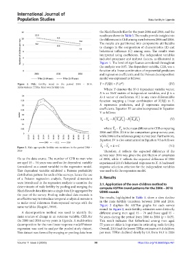
Figure 2. Male fertility trend in the period 2006 – 2016. Y = F(Xβ) = F (e ) (IV)
Abbreviations: TFRm: Male total fertility rate.
Where Y denotes the N×1 dependent variable vector,
X is an N×K matrix of independent variables, and β is a
K×1 vector of coefficients. F(·) is any once-differentiable
function mapping a linear combination of X(Xβ) to Y.
X represents predictors, and β represents regression
coefficients. Equation IV can also be expressed in Equation
V as follows:
FX

Y Y A A FX (V)
B
A
B
B
where Y – Y is the mean difference in CEB comparing
B
A
2016 and 2006. 2016 is the comparison group survey year,
while 2006 is the reference group survey year. Furthermore,
Equation IV is also summarized in Equation VI as follows:
Y Y EC (VI)
Figure 3. Male age-specific fertility rate variations in the period 2006 – B A
2016 Therefore, E reflects the expected difference if the
survey year 2016 was given the distribution of covariates
file as the data source. The number of CEB to men who of 2006, while C reflects the expected difference if 2006
are aged 15 – 54 years was used as the dependent variable experienced 2016’s behavioral responses to X. A backward
(considered as a count variable) in the regression model. stepwise selection criterion for the independent variables
This dependent variable exhibited a Poisson probability was used to fit the regression model.
distribution pattern for each of the surveys, hence the use
of a Poisson regression analysis. Temporal dimensions 3. Results
were introduced in the regression analysis to examine the 3.1. Application of the own-children method to
determinants of male fertility by pooling and merging the compute ASFRm trend patterns for the 2006 – 2016
Man’s Recode data files into a single data file aggregated by UDHS rounds
the year of the survey. Pooling individual data records is
an effective way to introduce temporal analysis dimensions The results, highlighted in Table 1, show a slow decline
to make trend inferences from repeated surveys with the in the male fertility transition between 2006 and 2016.
same variables (Ruspini, 1999). Figure 3 displays the ASFRm graphs for each survey
round. In Figure 2, male fertility estimates were distinctly
A decomposition method was used to identify the different among men aged 15 – 79 and those aged 15 –
main sources of change in an outcome variable, CEB, for 54 years during the period from 2006 to 2016 (p > 0.05).
the 2006 and 2016 survey years in Uganda. A multivariate This result indicates that fatherhood among men aged
decomposition for the non-linear response model Poisson 55 years or older is important in estimating male fertility.
regression was used to analyze the pooled study dataset. Overall, 2016 had the lowest TFRm estimate at 8.4 children
This dataset was formed by merging or pooling data from per man. TFRm declined slowly by 1.9, from 10.3 in 2006

Volume 11 Issue 3 (2025) 98 https://doi.org/10.36922/ijps.461