Page 49 - IJPS-2-1

Akansha Singh and Laishram Ladusingh

Figure 1. Fitting of ln( n q x ) values using the Heligman–Pollard equation on SRS Data for males and females in India, at two time periods.

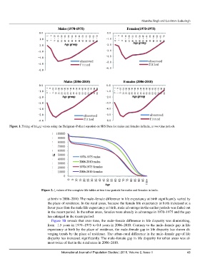
Figure 2. l x values of the complete life tables at two time periods for males and females in India.

at birth in 2006–2010. The male–female difference in life expectancy at birth significantly varied by
the place of residence. In the rural areas, because the female life expectancy at birth increased at a
faster pace than the male life expectancy at birth, male advantage in the earlier periods was faded out
in the recent period. In the urban areas, females were already in advantage in 1970–1975 and the gap
has enlarged in the recent period.
Figure 3B reveals that over time, the male–female difference in life disparity was diminishing,
from −1.5 years in 1970–1975 to 0.4 years in 2006–2010. Contrary to the male–female gap in life
expectancy at birth by the place of residence, the male–female gap in life disparity has shown di-
verging trends by the place of residence. The urban–rural difference in the male–female gap of life
disparity has increased significantly. The male–female gap in life disparity for urban areas was al-
most twice of that in the rural areas in 2006–2010.

International Journal of Population Studies | 2016, Volume 2, Issue 1 43