Page 47 - IJPS-2-1

Akansha Singh and Laishram Ladusingh

from age x to x+1) using the parametric technique of Heligman and Pollard (1980) with the help of
Mortpak developed by United Nations Population Division (2003), which provides smoothed values
of 1q x. The parametric model provides a smoothed curve, which reaches the whole age interval and
provides flexible solutions in a set of parameters. This facilitates comparisons between and across
time periods and spaces (Kostaki and Panousis, 2001). The procedure for constructing a life table in
Mortpak from nm x or nq x is based on a method developed by Greville (1943). To construct a life table
with the open age group at 100+, the nq x values are extrapolated until no survivors remain, by fitting
a Makeham function through the last six nq x/(l − nq x) values available (United Nations Population
Division, 2003).
The conversion of age-specific death rates into age-specific probabilities of dying was consistent
with the RGI abridged life tables from 1970–1975 to 1991–1995. However, previous studies re-
ported problems in the conversion of age-specific death rates into age-specific probabilities of dying
at early ages in the recent SRS abridged life tables from 1996–2000 to 2002–2006 (e.g., Saikia,
Singh, and Ram, 2010). This conversion error further affects the estimates of infant, child mortality,
and the life expectancy at birth. The purpose of our new life tables from 1996–2000 to 2006–2010 is
to correct these errors. The nq x values of the newly constructed abridged life tables from 1996–2000
to 2006–2010 were used as inputs in the Heligman–Pollard equation. The complete life tables
were constructed according to 1q x values from age 0 to terminal age ω (100+).
2.3 Life Disparity

To measure dispersion of death, several measures such as S 10, interquartile range (Wilmoth and Ho-
riuchi, 1999), the Gini coefficient (Shkolnikov, Andreev, and Begun, 2003), the Theil index of in-
equality (Smits and Monden, 2009), and average interindividual difference and the related measures
of absolute inequality (Moser, Shkolnikov, and Leon, 2005; Shkolnikov, Andreev, and Begun, 2003)
are often used extensively. S 10 is defined as the standard deviation of the age at death for ages 10 or
older (Edwards and Tuljapurkar, 2005). The distance between the lower and the upper quartile of the
distribution of ages at death in a life table is called as interquartile range (Wilmoth and Horiuchi,
1999). The Gini coefficient is defined as the average of absolute differences in individual ages at
death relative to the average length of life (Shkolnikov, Andreev, and Begun, 2003). The inequality
in the distribution of age at death can be measured using the Theil index of inequality (Smits and
Monden, 2009). Some formal properties of these measures are different from each other and the de-
gree of their aversion to inequality. In this study, life disparity based on the distribution of death at
different ages was used to measure the dispersion of deaths. The convergence of death rates in a
narrow age interval can be observed from the decline in life disparity. The life disparity declines
when saving lives occur at early ages, which compresses the distribution of deaths. The distribution
of death expands when saving lives occur at late ages, which leads to increase in the average re-
maining life expectancy. Unlike life expectancy at birth, life disparity combines the age pattern of
mortality and average mortality in a single measure (Singh and Ladusingh, 2013). The concept of
this measure is in line with Keyfitz's idea that everybody dies prematurely, that is, every death de-
prives the individual concerned of his or her remaining life expectation (Keyfitz, 1977). Hence, life
disparity occurs because of deprivation from death and inequality in the length of life. The measure
of life disparity , appeared in several previous studies (Mitra, 1978; Zhang and Vaupel, 2009;
†

Shkolnikov, Andreev, Zhang, et al., 2011).
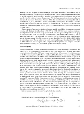
Life expectancy at age x is measured using the following formula:
0
e = T x (1)
x
l x
Life disparity at age x is estimated using the following formula:
∑
†
1 a 
e = 1 ω 1 − d  y ( y+ 1 +− y ) + 1 d ω  1 e ω    (2)
e
x
l x yx   l ω  2 
=
International Journal of Population Studies | 2016, Volume 2, Issue 1 41