Page 51 - IJPS-6-1

Acharya and Das

of rupees, whereas the area under forest cover is defined as the percentage of total geographical area. More importantly,
the normalization process provides us with the opportunity to estimate the single value and to comprehend the relationship
thereof. The selection of the indicators for preparing a composite index depends on the nature of the relationship of the
respective indicator with the predictor.
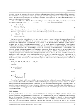
Let represent the value of the i climate vulnerability indicator in the j district if is positively associated with
th
th
ij
ij
the climate vulnerability (i = 1, 2, 3, ……., 10; j = 1, 2, ………, 10). Let us write the equation as:
X Min X
j
ij
ij
Y MaxX MinX ij (1)
ij
j
ij
j
Where Min and Max are the minimum and maximum of , respectively.
j
ij
j
j
i
However, if is negatively associated with climate vulnerability, equation (1) can be written as:
ij
MaxX X
j
ij
Y MaxX ij MinX ij (2)
ij
j
j
ij
Scaling the dimension index values, vary from zero (0) to one (1), where 0 indicates the lowest vulnerability and
ij
1 indicates the highest vulnerability. In all parameters, no normal or goalpost value has been defined. The observed
maximum value of parameters has been taken as the goalpost value, and the observed minimum value is taken as a
minimum from the matrix of scaled dimension values, Y = {(Y )}. In this process, we constructed the “Composite Index
ij
of Climate Vulnerability” for different districts of Odisha. The above-mentioned method is quite like the United Nations
Development Programme’s HDI. The Ministry of Science and Technology also uses the method – Government of India
under the National Mission for Sustaining the Himalayan Ecosystem as part of National Action Plan on Climate Change
to develop the Climate Vulnerability Assessment of Indian Himalayan Region (DST-GoI, 2018-2019). Further, we have
assigned the weights of the indicators using principal component analysis. The weight is also generated in view of the
importance of indicator on determining climate vulnerability and its effect on agriculture production. While assigning the
weight, it was ensured that the weight or proportion assigned to all the indicators add up to “1;” where, the weight W, of
the i indicator, varies inversely as the variation in the respective indicator of climate vulnerability status subject to the
th
condition:
0 W i 1 and W 1 W 2 W 3 ........ W m 1
Such that,
K
W =
i
VarianceY i (3)
Where,
m 1 1
K
i 1 VarianceY i (4)
The choice of weights in this manner is taken up to ensure that large variations in any one of the indicators will not
unduly dominate the contribution of the rest and distort the inter-group comparisons across the districts. To obtain a
weighted average of a composite aggregated index value, we have added the total weighted value of each indicator of the
same district and the sum is divided by the total number of indicators of the same district. The signs of the indicators (+ve
or −ve) are assigned accordingly based on the fact whether each of them is contributing to an increase in or decrease in
climate vulnerability.
2.2.3. Methods
To investigate the effects, we have used a correlation matrix and the techniques of multiple regression analysis. Under
multiple regressions, six different models (four models for child nutrition and two for women nutrition) are used to
find out the association. Following two types of regression models are worked out to identify the factors responsible
for determining the household nutritional status in Odisha. We define the (HNS) Household Nutrition Status as listed
below with three indicators, BPI as Biophysical Indicators (five indicators as mentioned in Table 1), SEI defined as

International Journal of Population Studies | 2020, Volume 6, Issue 1 45