Page 10 - IJPS-9-1

International Journal of
Population Studies Local population changes as a spatial varying multiscale process

zero-centered and based on the same range of variation. the country. It is important to underline that, if we refer to the
Consequently, the bandwidths are unconstrained from the Italian population only (i.e., people with Italian citizenship), the
scale and the variation of the explanatory variables, helping decrease was even sharper, from 55,847,162 million residents
the relative comparison of bandwidths (Oshan et al., 2020). to 54,820,515 (a total decline by −18.3‰), proving the growth
In the first phase, we built a classic ordinary least square of the foreign population counterpart, from 4,101,335 to
(OLS) model (which assumes processes to be constant 4,966,158 (a total increase by +210.9‰).
across the study area) as a benchmark for evaluation of The results of global (OLS) and local (MGWR)
the MGWR model and report comparison. Before moving regression models are clear (Table 1). The first important
to the presentation of the results, it should be noted one finding is that, based on the Monte Carlo randomization
limitation of the present study. The independent variables significance test for spatial variability, all the variables
used (demographic rates obtained by a decomposition introduced in the model are affected by spatial variability
approach) can interact with each other. The estimation done so that it would be misleading to treat them as constant in
cannot grasp this (possible) effect of interaction between space (like in the OLS model). Moreover, they are supposed
independent variables. Nevertheless, our primary goal here to be not correlated because the variance inflation factor
is not to understand the “net” effect of the independent (VIF) value is always lower than 10.
variables on the dependent one nor to explain the variance
of this latter. Our primary goal is to prove that the local MGWR outperforms the OLS model: AICc is lower,
demographic change in Italy is a local multiscale process Adj-R-square is higher, and the distribution of residuals is
(i.e., it varies across spaces and across scales). not spatially autocorrelated (see the not significant value of
the I _MGWR_res respect to the significant value of the I _OLS_res
3. Key Findings in Table 1). OLS results tell us that all the independent
From 2011 (January 1) to 2019 (January 1), the resident variables are statistically significant. The net effect on the
population in Italy passed from 59,948,497 to 59,816,673 (a dependent variable is always positive. NATPGR has a
decline by −2.2‰). Those changes present a strong spatial higher net impact, followed by MIGPGR.
variation as clearly shown in Figure 1. The right panel map What is important, in our view, in addition to the spatial
clearly shows a sort of “broken” space that divides local contexts variability of the local coefficients, is the variation of the
that recorded an increase of resident population during 2011 – scale (i.e., the bandwidth) for each regression coefficient.
2019 from the other. The positive growth areas are most of the In the case of adaptive kernel, the bandwidth represents
cases represented by urban areas and big cities mainly located the number of nearest neighbors from the regression point
in the center and northern Italy (like Milan, Bologna, Florence, which receives a non-zero weight in the local regressions
Rome) while the negative growth areas are represented by (i.e., the ones which are considered as neighbors to i). The
inner contexts but also by some important medium and selection of the optimal bandwidth parameters is based on
medium-large cities mainly located in the southern part of statistical optimization criteria like Akaike Information

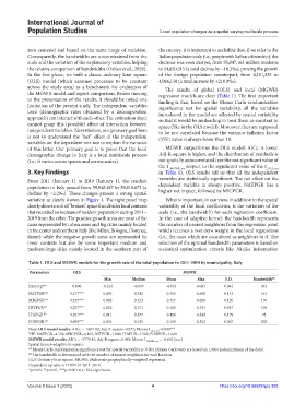
Table 1. OLS and MGWR models for the growth rate of the total population in 2011‑2019 by municipality, Italy

Parameters OLS MGWR
Min Median Mean Max S.D. Bandwidth (b)
Intercept (a) 0.000 -0.162 -0.007 -0.032 0.083 0.061 361
NATPGR (a) 0.477*** 0.093 0.342 0.355 0.649 0.133 161
MIGPGR (a) 0.455*** 0.082 0.323 0.327 0.668 0.120 170
INTPGR (a) 0.227*** 0.025 0.171 0.165 0.343 0.057 105
ITAPGR (a) 0.281*** 0.011 0.477 0.458 0.848 0.179 78
FORPGR (a) 0.099*** 0.034 0.155 0.159 0.302 0.067 202
Note: OLS model results: AICc = -5691.82; Adj-R-square=0.972; Moran I _OLS_res =0.034***
VIF: NATPGR=4.154; MIGPGR=4.165; INTPGR=1.800; ITAPGR=7.582; FORPGR=1.628
MGWR model results: AICc = -9779.45; Adj-R-square=0.985; Moran I _MGWR_res = -0.002 (n.s.)
Spatial kernel=adaptive bi-square
(a) Monte Carlo randomization significance test for spatial variability p<0.001 (Monte Carlo tests are based on 1,000 randomizations of the data)
(b) The bandwidth is determined with the number of nearest neighbors for each location
OLS: Ordinary least square. MGWR: Multiscale geographically weighted regression.
Dependent variable is TOTPGR 2011–2019.
*p<0.05; **p<0.01, ***p<0.001 n.s.: Not significant.

Volume 9 Issue 1 (2023) 4 https://doi.org/10.36922/ijps.393