Page 87 - JCAU-7-1

Journal of Chinese
Architecture and Urbanism Machine-simulated scoring of child-friendly streets

poor performance on new data), while the kernel function may be perceived as less desirable. In addition, cars had a
enabled the model to manage non-linear relationships in slight negative correlation with predicted scores (-0.089,
the data. In addition, the gamma parameter and epsilon p<0.01), reflecting the negative effect of motor vehicles
tolerance fine-tuned the accuracy and error tolerance of on perceived safety.
the model’s predictions. The correlation heat map (Figure 7) visually illustrates
5. Analysis and results the strength and direction of correlations between
features and predicted scores, with colors ranging from
5.1. Feature-score correlations blue (negative correlation) to red (positive correlation).

To investigate the relationships between perception A strong positive correlation (0.94) between “tree_
scores and SVI features, a Spearman correlation analysis plant_grass” and “predicted score” indicates that green
was conducted, considering both data characteristics coverage has a significant impact on predicted scores,
and analysis objectives. This method helps to understand while a strong negative correlation (-0.59) between
how different variables interact and influence the “building” and predicted scores indicates that places
predicted scores for street child-friendliness, uncovering with more buildings have lower predicted scores. The
correlations for “person” (-0.21) and “sky” (0.12) were
the relationship between multiple environmental weaker, indicating a limited direct impact on predicted
features and predicted scores. Spearman correlation was scores.
chosen as it does not assume linear relationships, unlike
other correlation measures. Variance inflation factor In contrast to the correlation heat map, the scatter plot
checks were performed, as Spearman correlation does (Figure 8) provides visual evidence of the distribution
not assume or assess linearity between variables. Table 2 of different eigenvalues above and below the predicted
illustrates inter-variable correlations, identifying key and median score. The blue portion of the graph represents
redundant features that influence the perceived child- scores above the median, while the red portion represents
friendliness of streets and clarifies how each variable scores below it.
impacts prediction scores to guide model refinement. The analysis shows that subjective perceptions of safety
For instance, a strong positive correlation (0.937, are lower in areas with higher pedestrian and vehicle
p<0.01) was observed between natural elements (trees, elements, potentially due to noise and traffic, which can
plants, and grasses) and perceived safety, suggesting be disruptive, especially for children. The influence of
that more natural elements enhance perceived safety. architectural and sky elements on the predicted scores
Streetlights also positively correlated with the score appears more uniform, with higher scores associated with
(0.157, p<0.01), especially at night, when streetlights fewer architectural elements in the streetscape, suggesting
contribute to safety. In contrast, buildings showed a that open views positively correlate with the subjective
significant negative correlation with predicted scores experience of health and safety. In addition, the scatter plot
(-0.589, p<0.01), suggesting that urban environments (Figure 8) shows that areas rich in greenery tend to have

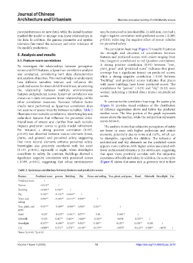
Table 2. Spearman correlations between features and predictive scores

Feature Predicted score person Building Sky Fence and railing Tree, plant, and grass Road Sidewalk Streetlight Car
Predicted score 1
Person −0.211** 1
Building −0.589** 0.503** 1
Sky 0.120** −0.434** −0.609** 1
Fence and 0.090** −0.203** −0.314** 0.306** 1
railing
Tree, plant, and 0.937** −0.189** −0.508** 0.063* 0.251** 1
grass
Road 0.027 −0.133** −0.131** 0.277** −0.02 −0.143** 1
Sidewalk 0.023 0.417** 0.463** −0.428** −0.162** 0.034 −0.255** 1
Streetlight 0.157** −0.104** −0.233** 0.351** 0.180** 0.132** 0.108** −0.055 1
Car −0.089** 0.271** 0.371** −0.316** −0.179** −0.075* −0.116** 0.206** −0.035 1
Notes: *p<0.05, **p<0.01.

Volume 7 Issue 1 (2025) 10 https://doi.org/10.36922/jcau.3578