Page 45 - MSAM-2-1

Materials Science in Additive Manufacturing Data imputation strategies of PBF Ti64

variables in a sequential fashion such that prior imputed
values are used as part of the model in predicting
subsequent variables. Hence, each variable can be modeled
conforming to its distribution with continuous variables
modeled using linear regression, while binary variables are
modeled with logistic regression.
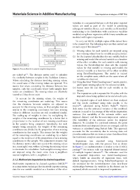
To carry out MICE, multiple copies of the dataset have
to be created first. The following steps are then carried out
on each copy of the dataset :
[29]
(i) Missing values for each variable are imputed using
non-missing values from the variable as a placeholder.
(ii) Set the imputed placeholders for one variable back to
missing and model the selected variable as a function
of the other variables. For each variable with missing
values, the IterativeImputer class sets the imputed
values for that variable to missing and models the
Figure 2. Process flow for k-nearest neighbor imputation.
selected variable as a function of the other variables
using ExtraTreesRegressor. The model is trained
are scaled-up . The distance metric used to calculate
[27]
the similarity between samples is the Euclidean distance. on the complete cases, which are the cases where all
When calculating the distance involving missing values, variables are observed.
the coordinates of the missing values are ignored. This (iii) Using the fitted “ExtraTreesRegressor” model, predict,
means that when calculating the distance between two and impute missing values for the selected variable.
samples, only the coordinates where both samples have (iv) Repeat steps (ii) and (iii) for each variable in the
values are considered. The missing values are effectively dataset.
treated as if they do not exist. (v) The imputation cycle is repeated for 10 cycles, with the
imputed values being updated at the end of each cycle.
To account for the missing values, the weights of
the remaining coordinates are scaled-up. This means The imputed copies of each dataset are then analyzed
that the distances between samples are adjusted to and the results combined using rules specific to the
[28]
[30]
account for the missing values, so that samples that are results , calculated using Rubin’s Rules . Rubin’s
similar in the remaining coordinates but have missing Rule states that the estimated variance of the combined
values in different locations are still considered similar. estimate is equal to the average of the within-imputation
The scaling-up of weights is done by multiplying the variance (the variability of the estimate within each
weights of the remaining coordinates by a factor that is imputed dataset) and the between-imputation variance
proportional to the number of non-missing coordinates (the variability of the estimates across the imputed
in the samples being compared. Specifically, for each datasets). To calculate the combined estimate, the point
sample being compared, the weights of the remaining estimates from each imputed dataset are averaged, and the
coordinates are divided by the proportion of non-missing variance is calculated using Rubin’s Rule. This approach
coordinates in that sample. This means that the weights accounts for the uncertainty due to missing data and
of the remaining coordinates are scaled-up by a factor provides estimates that are more accurate than those from
equal to the reciprocal of the proportion of non-missing the traditional complete case analysis.
coordinates in the sample. This adjustment ensures that Imputation was executed using Sckit-learn’s
the distance metric takes into account the missing values IterativeImputer class, with the process flow as shown
in a meaningful way, without allowing the missing values in Figure 3. Its implementation is similar to the R MICE
to dominate the calculation. Each sample’s missing values package but returns only one imputed dataset instead
[28]
are imputed using the mean value from n_neighbors of multiple imputed datasets . The estimator used for
[31]
nearest neighbors, with n_neighbors = 5. the sequential imputation was ExtraTreesRegressor,
which builds an ensemble of regression trees, with
2.1.2. Multivariate imputation by chained equations default hyperparameters. Using ExtraTreesRegressor as
Multivariate imputation by chained equations (MICE) the estimator for the IterativeImputer class, non-linear
[28]
is an imputation technique that iteratively imputes missing relationships between the variables in the dataset can be
data for one variable modeled as a function of the other captured, which can result in improved imputations.

Volume 2 Issue 1 (2023) 4 https://doi.org/10.36922/msam.50