Page 46 - MSAM-2-1

Materials Science in Additive Manufacturing Data imputation strategies of PBF Ti64

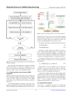
Figure 4. Schematics of graph imputation neural network imputation .
[27]
missing values . Pruning is carried out twice by dropping
[33]
all the connections below the 97.72 percentile, which was
th
found to be a good value from experimental tests , for
[33]
each row, leaving behind the most relevant nodes.
The graph convolution autoencoder used is defined as:
H=ReLU LX (II)

1
ˆ
X=Sigmoid (LH Θ 2 ) (III)
Equation II is the encoder that takes the input X,
with L as the Laplacian matrix related to the graph, and
Θ as a matrix of adjustable coefficients, and produces an
1
encoded value H. Equation III is the decoder that provides
ˆ
a reconstructed imputed dataset X from the encoded H.
The graph convolution network is trained to minimize
the loss function arising from errors in reconstruction as
defined below:
Figure 3. Process flow for graph imputation neural network imputation
using IterativeImputer. ˆ ˆ
L = α MSE ( X,X ) (1+ − α ) CE(X,X) (IV)
A
Since the Extra Trees algorithm is similar to Random
Forest, which does not make any assumptions on the Where MSE is the mean squared error for numerical
data , the distribution of the dataset to be imputed would variables, CE is the cross-entropy for categorical variables,
[32]
not have a major impact on the imputation result. and is an additional hyperparameter set as the ratio
between numerical and categorical variables .
[33]
2.1.3. Graph imputation neural network (GINN)
imputation Adversarial training of the autoencoder is used in which
a feedforward network is used as the critic to differentiate
GINN is a deep learning library that imputes missing data between imputed and non-imputed data, introducing an
by first building a graph of similarities between complete additional term to the loss function to include adversarial
values and then running an autoencoder with graph loss . A more in-depth explanation of the GINN
[33]
convolutions on top of that, with the schematics shown in framework can be found in a previous work .
[33]
Figure 4 .
[33]
2.2. Cleaning of the dataset
To develop the graph of similarities, each node of the
graph is represented by a feature vector in the dataset, with Since there is a significant proportion of missing data
Euclidean distance used to find the similarity between non- in the dataset, initial data cleaning has to be carried out

Volume 2 Issue 1 (2023) 5 https://doi.org/10.36922/msam.50