Page 30 - TD-3-1

Tumor Discovery AI uncovers tumor spatial organization

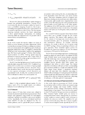
LL recon L KL an extensive study utilizing this data, encompassing spot-
level information, layer-level data, and spatial marker
25
pZ))
L qZ(| ,)XA [log p AZ (| )] KL qZ XA(( |, )||( (V) genes. The project comprises a total of 12 samples, each
dissection covering six neuronal layers plus white matter.
Consequently, eight samples were categorized into seven
The term KL(.) denotes the Kullback-Leibler divergence
between two probability distributions. Training VGAE clusters, while the remaining four were grouped into five
(ground-truth, cortical layers one to six, white matter).
to minimize this objective function enables the model to For validation of the GNN algorithm, sample 151673 was
learn a probabilistic mapping of spots to a latent space,
facilitating meaningful and informative representations of chosen as a representative due to its specificity. This sample
the structure and features of the ST data. The downstream entails 3,639 spots and 33,538 genes, with provided spot
clustering methods partition the latent embeddings annotations.
to detect spatial domains. Subsequently, the resulting The second ST dataset originates from human breast
clustering labels are compared with the ground-truth to cancer tissue and is available through the 10× Visium
assess accuracy and performance. dataset repository. This dataset holds significant value
for the analysis of heterogeneous tumor and immune
2.2. GNN microenvironments, given its substantial intratumoral
In the VGAE model, the encoder utilizes two layers of and intertumoral variations. To facilitate clustering
GNNs to extract features and reduce dimensions. GNNs estimation, the sample is divided into 20 regions using
26
facilitate the processing of ST data by enabling spots to learn the SEDR package, relying on pathological features and
from and communicate with neighboring spots. Each spot gene expression. These annotated regions provide the
aggregates information from its neighbors, subsequently foundation for clustering evaluation. In total, this dataset
updating its own representation based on this aggregated encompasses 3798 spots and 36,601 genes.
data. The Pytorch_pyG package in Python offers multiple The 10× Xenium technology represents a novel approach
23
implementations of GNNs. Existing spatial clustering integrating single-cell, spatial, and in situ analysis of FFPE
architectures typically incorporate only a single GNN. In tissue. Notably, breast cancer tumor datasets associated
this study, we opt for the simple graph convolution (SGC) with this technology were reprocessed and republished
ConvNet to construct the encoder. on December 6, 2022. Leveraging its non-destructive
24
9
The SGC ConvNet highlights issues of model complexity workflow, Xenium spatially aligns RNA, protein, and
and redundant computations within GDL. To address these histological data within a unified image. This feature
defects, SGC ConvNet aims to minimize collapsing weight empowers us to discern cell types and their corresponding
matrices and nonlinearities between successive layers. gene expression profiles at a single-cell resolution. In the
This streamlined linear model demonstrated comparable breast cancer tumor dataset, a remarkable seventeen
or even superior performance at both theoretical and distinct cell types have been identified, amounting to
experimental levels. Notably, the convolution kernel in 164,079 cells and utilizing a 313-plex gene panel. To alleviate
SGC is redefined as a linear function (Equation VI): computational load, this manuscript employs a segmented
version of this data for clustering comparison, comprising

K
()1

Y ˘ SGC soft max ...S SSX ()2 ... ()K soft max SX 15 cell types, 11,996 cells, and the 313 gene panel.
(VI) 2.4. Data pre-processing and hyperparameters
where S is the normalized adjacent matrix, X is the In this article, data pre-processing and VGAE training
feature matrix, Θ is the weight matrix, and softmax are conducted within a Python virtual environment using
indicates the normalized exponential function. PyTorch_pyG, Squidpy, and Scanpy toolkits. Initially,
gene expression profiles undergo normalization and log
2.3. ST datasets transformation using Scanpy. Users also have the option
27
Various types of ST data from tumors were utilized to to select “SCTransform” for gene expression normalization.
evaluate the proposed spatial clustering architecture. These Three thousand highly variable genes are selected to
datasets were generated using diverse ST technologies, construct the feature matrix. Subsequently, the scikit-learn
resulting in variations in resolution, spot counts, and gene toolkit employs a nearest-neighbor search technique to
28
profiles. Specifically, the human dorsolateral prefrontal calculate the adjacency matrix. The neighbors for each
cortex (DLPFC) ST data was obtained from the 10× spot are determined using either the k-nearest neighbor
Visium platform, and the spatialLIBD project conducted or radius-nearest neighbor modes. Specifically, for the 10×

Volume 3 Issue 1 (2024) 4 https://doi.org/10.36922/td.2049