Page 43 - AIH-2-4

Artificial Intelligence in Health ViT for neurodegeneration diagnosis

3.3. Data pre-processing performance using ViTs. However, most large computer vision

The F-FDG PET scans in the ADNI dataset were acquired datasets include natural images with three RGB channels.
18
utilizing different types of imaging devices and during various Therefore, we reshaped the samples to 3 × 570 × 950 in our
phases. Therefore, these scans vary significantly in their dataset to utilize transfer learning and available pre-trained
models. This procedure constructs a three-channel image,
properties, including the image size, number of channels, in which every channel depicts the brain along a unique axis
and intensities of voxels. Furthermore, they include the (sagittal, coronal, and axial). Figure 2 shows the result of data
subject’s skull, which does not deliver beneficial information pre-processing and reshaping steps on a single scan.
regarding NDD diagnosis. Furthermore, raw scans may
contain noise or blur due to the patient’s movement or other 3.5. Model architecture and training
technical issues. Consequently, we use the pre-processing
procedure developed by Etminani et al., which employs Our proposed model has a similar architecture to vanilla
4
ViT, as suggested by Dosovitskiy et al. After training
6
MATLAB and statistical parametric mapping (SPM12) different models with and without transfer learning,
33
32
to ensure all scans have the same properties.
we concluded that pre-training is crucial to obtaining
The pre-processing steps for each sample are as follows: excellent results. Therefore, we employed the Hugging
• We converted the scan to the NIfTI format Face Transformer API and model hub for development.
34
• It was crucial to place the brain approximately in Specifically, the foundation of our model is a base-sized
the center of the scan. Therefore, we reoriented and ViT, pre-trained on ImageNet-21k and ImageNet 2012,
36
35
repositioned the brain to set the volume’s origin at the respectively. Finally, we fine-tuned the model on our F-
37
18
anterior commissure region FDG PET scan dataset to classify NDDs.
• Our dataset included scans of various shapes. Hence, Figure 3 illustrates the model’s diagram, inspired by
we normalized the scan to ensure all samples had Dosovitskiy et al. First, the scan was resized to 3 × 384 ×
6
identical spatial size and number of channels 384 to match the model’s input shape. Then, the scan was
• Using the tissue probability map of SPM12, the brain divided into patches of 3 × 32 × 32, flattened, and supplied
was segmented to a standard transformer along with position embeddings
• The last pre-processing stage removed the subject’s holding the spatial information. Finally, a multilayer
skull from the scan. Consequently, we used perceptron head translated the model’s final hidden state
segmentation maps obtained from the previous step into the probability of classes for the classification task.
with a filter for skull-stripping. Table 2 summarizes the model’s specifications.
The pre-processing procedure led to skull-stripped scans We employed an AdamW optimizer (learning rate = 5e-5,
of size 79 × 95 × 79, representing channels, height, and width, weight decay = 0.15) for model development. Furthermore, an
respectively. Then, the values of voxels were normalized using exponential learning rate decay (γ = 0.9999 per epoch) was used
a min-max scaler across the channels in Python. Finally, we during training. Finally, we selected a weighted cross-entropy
dismissed the initial ten and last nine channels of the 3D scan as the loss function, in which the weight of each class was the
since they included a tiny fraction of the brain, resulting in inverse of its frequency during training, as shown below:
3D scans with the shape of 60 × 95 × 79.
l (x,y) = L = {l ... l } ⊺ (I)
1
N
3.4. Data reshaping C exp(x )
, n c
According to our experiments and the literature, pre-training l = − ∑ c= 1 w c log ∑ C exp(x ) y , n c
6
n
on large amounts of data is crucial to achieving the best i= 1 , ni (II)
A B C

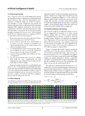
Figure 2. After the initial data pre-processing, we reshaped each scan of 60 × 95 × 79 to a three-channel image of 3 × 570 × 950, in which every channel
illustrates the brain along a unique axis. This data reshaping was crucial to utilize transfer learning and pre-train the model on large computer vision
datasets that contain natural three-channel RGB images. (A) Sagittal, (B) Coronal, (C) Axial.

Volume 2 Issue 4 (2025) 37 doi: 10.36922/AIH025140026