Page 140 - AJWEP-22-5

Messel, et al.

)( −
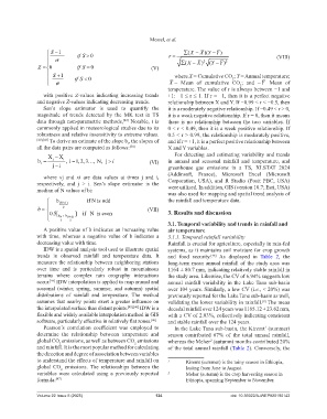
 S − 1 ∑ (X − XY Y )
 σ 0if S > r = (VIII)
−
 ∑ (X − X ) 2 (YY ) 2
0 if S =
Z =  0 (V)
 S + 1
 if S < 0 where X = Cumulative CO ; Y = Annual temperature;
2
 σ X = Mean of cumulative CO ; and =Y Mean of
2
temperature. The value of r is always between −1 and
with positive Z-values indicating increasing trends +1: −1 ≤ r ≤ 1. If r = −1, then it is a perfect negative
and negative Z-values indicating decreasing trends. relationship between X and Y. If −0.99 < r < −0.5, then
Sen’s slope estimator is used to quantify the it is a moderately negative relationship. If −0.49 < r > 0,
magnitude of trends detected by the MK test in TS it is a weak negative relationship. If r = 0, then it means
data through non-parametric methods, Notable, t is there is no relationship between the two variables. If
[42]
commonly applied in meteorological studies due to its 0 < r < 0.49, then it is a weak positive relationship. If
robustness and relative insensitivity to extreme values. 0.5 < r > 0.99, the relationship is moderately positive,
[40],[43] To derive an estimate of the slope b , the slopes of and if r = +1, it is a perfect positive relationship between
all the data pairs are computed as follows: i [34] X and Y variables.
X − X For detecting and estimating variability and trends
b = j i , i 1, 2, 3 , N, j i (VI) in annual and seasonal rainfall and temperature, and
…
>
=
i
j i − greenhouse gas emissions in a TS, XLSTAT 2024
(Addinsoft, France), Microsoft Excel (Microsoft
where xj and xi are data values at times j and i,
respectively, and j > i. Sen’s slope estimator is the Corporation, USA), and R Studio (Posit PBC, USA)
median of N values of bi: were utilized. In addition, GIS (version 10.7; Esri, USA)
was also used for mapping and spatial trend analysis of
 b (N 1)+ if N is odd the rainfall and temperature data.

b =  2 (VII) 3. Results and discussion
 0.5[ b N + b ( N 2)+ ] if N is even
 2 2
3.1. Temporal variability and trends in rainfall and
A positive value of b indicates an increasing value air temperature
with time, whereas a negative value of b indicates a 3.1.1. Temporal rainfall variability
decreasing value with time. Rainfall is crucial for agriculture, especially in rain-fed
IDW is a spatial analysis tool used to illustrate spatial systems, as it maintains soil moisture for crop growth
trends in observed rainfall and temperature data. It and food security. As displayed in Table 2, the
[48]
measures the relationship between neighboring stations long-term mean annual rainfall of the study area was
over time and is particularly robust in mountainous 1164 ± 80.7 mm, indicating relatively stable rainfall in
terrains where complex rain orography interactions the study area. Likewise, the CV of 6.94% suggests low
occur. IDW interpolation is applied to map annual and annual rainfall variability in the Lake Tana sub-basin
[44]
seasonal (winter, spring, summer, and autumn) spatial over 104 years. Similarly, a low CV (i.e., < 20%) was
distributions of rainfall and temperature. The method previously reported for the Lake Tana sub-basin as well,
assumes that nearby points exert a greater influence on validating the lower variability in rainfall. The mean
[8]
the interpolated surface than distant points. [45],[46] IDW is a decadal rainfall over 124 years was 1165.12 ± 23.62 mm,
flexible and widely available interpolation method in GIS with a CV of 2.03%, collectively indicating consistent
software, particularly effective in relatively flat zones. [46] and stable rainfall over the 124 years.
Pearson’s correlation coefficient was employed to In the Lake Tana sub-basin, the Kiremt (summer)
1
determine the relationship between temperature and season contributed 67% of the total annual rainfall,
global CO emissions, as well as between CO emissions whereas the Meher (autumn) months contributed 20%
2
2
2
and rainfall. It is the most popular method for calculating of the total annual rainfall (Table 2). Conversely, the
the direction and degree of association between variables
to understand the effects of temperature and rainfall on 1 Kiremt (summer) is the rainy season in Ethiopia,
global CO emissions. The relationships between the lasting from June to August.
2
variables were calculated using a previously reported 2 Meher (autumn) is the crop harvesting season in
formula: [47] Ethiopia, spanning September to November.

Volume 22 Issue 5 (2025) 134 doi: 10.36922/AJWEP025190142