Page 160 - {PDF Title}

Mhaske and Kumar

72
MST 45.  5 (II)
2
In Table 2, the frequent items are identified as Items
A and B, with a value of seven each, surpassing the MST
of 5. Likewise, Item C has a value of 6 that surpasses
the MST. Subsequently, an array is formed to store these
frequent items. Based on Table 2, the uncommon items
are eliminated. Subsequently, Table 3 shows a sample
dataset, and Table 4 reveals the sample dataset after
eliminating the uncommon items. 39
(ii) Generating combinations.
After eliminating the uncommon items, the
frequent items are united, as shown in Table 5.
After implementing the procedure of combination
generation, the following stage is dynamic itemset
counting.
(iii) Dynamic itemset counting:
The blank item sets are spotted with a solid box.
All the item sets are spotted in dashed rounds.
The transaction experimental values that
range from 1 to 55 are read and marked with
a dashed circle. When the count of dash circles
goes beyond the threshold, it turns into a dash
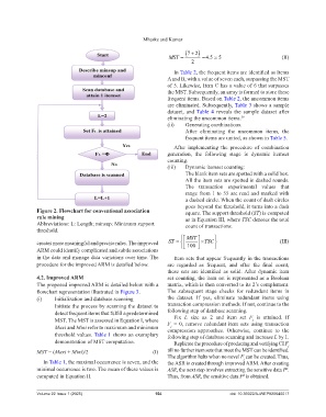
Figure 2. Flowchart for conventional association square. The support threshold (ST) is computed
rule mining as in Equation III, where TSC denotes the total
Abbreviations: L: Length; minsup: Minimum support count of transactions.
threshold.
MST
creates more meaningful and precise rules. The improved ST 100 TSC (III)
ARM could identify complicated and subtle associations
in the data and manage data variations over time. The Item sets that appear frequently in the transactions
procedure for the improved ARM is detailed below. are regarded as frequent, and after the final count,
these sets are identified as solid. After dynamic item
4.2. Improved ARM set counting, the item set is represented as a Boolean
The proposed improved ARM is detailed below with a matrix, which is then converted to its 2’s complement.
flowchart representation illustrated in Figure 3. The subsequent stage checks for redundant items in
(i) Initialization and database scanning the dataset. If yes, eliminate redundant items using
Initiate the process by scanning the dataset to transaction compression methods. If not, continue to the
detect frequent items that fulfill a predetermined following step of database scanning.
Fix L size as 2 and item set F is attained. If
MST. The MST is assessed in Equation I, where F = 0, remove redundant item sets using transaction
j
Maxi and Mini refer to maximum and minimum compression approaches. Otherwise, continue to the
j
threshold values. Table 1 shows an exemplary following step of database scanning and increase L by 1.
demonstration of MST computation. Replicate the procedure of producing and verifying CI F
j
MST = (Maxi + Mini)/2 (I) till no further item sets that meet the MST can be identified.
The algorithm halts when no novel F can be created. Thus,
j
In Table 1, the maximal occurrence is seven, and the the ASR is created through improved ARM. After creating
minimal occurrence is two. The mean of these values is ASR, the next step involves extracting the sensitive data P .
d
computed in Equation II. Thus, from ASR, the sensitive data P is obtained.
d

Volume 22 Issue 1 (2025) 154 doi: 10.36922/AJWEP025040017