Page 162 - {PDF Title}

Mhaske and Kumar

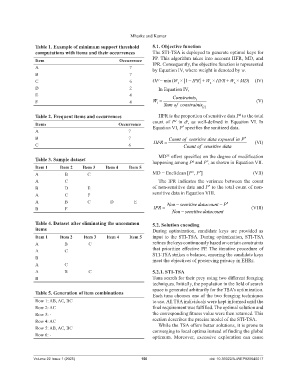
Table 1. Example of minimum support threshold 5.1. Objective function
computations with items and their occurrences The STI-TSA is deployed to generate optimal keys for
Item Occurrence PP. This algorithm takes into account HFR, MD, and
A 7 IPR. Consequently, the objective function is represented
by Equation IV, where weight is denoted by w.
B 7
C 6 OF = min (W × [1 − IPR] + W × HFR + W × MD) (IV)
2
1
3
D 2 In Equation IV,
E 4 Constraints
F 4 W i (V)
i
Sum of constraints i
d
Table 2. Frequent items and occurrences HFR is the proportion of sensitive data P to the total
d
s
Items Occurrence count of P in d , as well-defined in Equation VI. In
Equation VI, P specifies the sanitized data.
*
A 7
B 7 Count of sensitive data exposed inP
C 6 HFR Count of sensitive data (VI)
MD offers specifics on the degree of modification
38
Table 3. Sample dataset happening among P and P , as shown in Equation VII.
*
d
Item 1 Item 2 Item 3 Item 4 Item 5
*
D
A B C MD = Euclidean [P , P ] (VII)
A C The IPR indicates the variance between the count
*
B D E of non-sensitive data and P to the total count of non-
A C F sensitive data in Equation VIII.
A B C D E Nonsensitivedatacount P

B F IPR (VIII)
Nonsensitivedatacount

Table 4. Dataset after eliminating the uncommon 5.2. Solution encoding
items During optimization, candidate keys are provided as
Item 1 Item 2 Item 3 Item 4 Item 5 input to the STI-TSA. During optimization, STI-TSA
A B C refines the keys continuously based on certain constraints
A C that prioritize effective PP. The iterative procedure of
B STI-TSA strikes a balance, ensuring the candidate keys
meet the objectives of preserving privacy in EHRs.
A C
A B C 5.2.1. STI-TSA
B Tuna search for their prey using two different foraging
techniques. Initially, the population in the field of search
space is generated arbitrarily for the TSA’s optimization.
Table 5. Generation of item combinations
Each tuna chooses one of the two foraging techniques
Row 1: AB, AC, BC to use. All TSA individuals were kept informed until the
Row 2: AC final requirement was fulfilled. The optimal solution and
Row 3: - the corresponding fitness value were then returned. This
Row 4: AC section describes the precise model of the STI-TSA.
While the TSA offers better solutions, it is prone to
Row 5: AB, AC, BC converging to local optima instead of finding the global
Row 6: - optimum. Moreover, excessive exploration can cause

Volume 22 Issue 1 (2025) 156 doi: 10.36922/AJWEP025040017