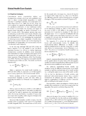
Page 183 - GHES-2-1

Global Health Econ Sustain Income-related inequality in health

2.3. Empirical strategies for the sample with a low mean (i.e., close to 0) than for

Concentration curves, concentration indices, and the sample with a high mean (i.e., close to 1). Therefore,
decomposition analysis, which are well-established tools the following corrected method developed by Erreygers
used to depict income-related inequalities in health (Erreygers, 2008) was used to calculate EI (Equation V):
outcomes in developed countries, were employed in this 4 µ
study (Bago d’Uva et al., 2009; Shin & Kim, 2010). The EI = (b −a ) CI (V)
tools compare the cumulative distribution of health with n n
the cumulative distribution of older individuals ranked where b and a represent the maximum and minimum
n
n
by income to demonstrate the direction and degree of of the dependent variable, i.e., SRH or ADL ability; μ is
income-related inequality in health (O’Donnell et al., the mean of SRH or ADL ability in the sample; and CI
2007; Gravelle, 2003). This method includes four steps: represents the CI specified in Equation IV. The value of
(i) estimating a model of the determinants of health using EI ranges from −1 to 1. A positive EI indicates that the
demographic and socioeconomic variables; (ii) calculating health variable is more concentrated among the rich, while
the unstandardized CI; (iii) calculating the standardized a negative EI indicates that the health variable is more
CI, showing income-related inequalities in health driven concentrated among the poor.
only by socioeconomic factors; and (iv) decomposing the The inequality EI is driven by both demographic
contribution of demographic and socioeconomic factors factors and socioeconomic factors. To identify only
from the total health inequality. socioeconomic-related differences in health, I used
In the first step, although SRH and ADL ability are indirect standardization to calculate inequalities in health
binary variables, it is not suitable to use non-linear only driven by socioeconomic factors (Kakwani et al.,
regression because it is difficult to further implement 1997). The process of standardized health variables is as
decomposition analysis. In addition, many researchers follows (Equation VI):
have found that the results of ordinary least square (OLS) = α y ˆ ˆ β + ˆ N γ + ˆ + ε Z
regression do not significantly differ from those of non- ∑ i ki ∑ k j ji i (VI)
linear regression (Yang & Kanavos, 2012; Van Doorslaer k j
et al, 2000). Therefore, OLS regression was used to identify where ˘ y represents the predicted value of health variables.
i
the determinants of SRH and ADL. The model is as follows As the equation shows, the actual values of the demographic
(Equation III): variables are used for standardization, while the mean values of
the socioeconomic variables are used as controls.
= α y ∑ i β + N ki ∑ k γ + j ji + ε Z i (III)
k j The indirectly standardized health variable was
calculated using the difference between the actual health
where y represents the actual health variables, i.e., variable (y ) and the predicted value of the health variable
i
i
SRH and ADL ability, N represents a set of demographic ( ˘ y ), adding the sample mean value of the health variable
i
k
factors, and Z represents a set of socioeconomic factors. ( y ), to find the distribution of health variables only
j
Further calculation of the CI was conducted to show associated with socioeconomic factors. Thus, a positive
income-related inequality in SRH and ADL ability by standardized EI indicates pro-rich inequality, while a
employing the method by O’Donnell et al. (Equation IV) negative standardized EI indicates pro-poor inequality
(2007): after controlling for demographic factors.
2 Decomposition analysis was adopted in the final step to
CI = cov(y ,R ) (IV)
µ it it calculate the contribution of each determinant to the total
inequality. The model is as follows (Equation VII):
where μ represents the mean of SRH or ADL ability in
the sample, y represents SRH or ADL ability by individual =   αµ C + DE ∑ β µ C + γ µ C   4
it
(i) and year (t), and R represents the individual’s rank  y y Nk Nk ∑ k j Zj Zj  (VII)
it
within the income distribution. A positive CI means that  k j 
there is pro-rich inequality, while a negative CI implies that where μ is the mean, k is a vector of variables (N ), j is a
k
there is pro-poor inequality. vector of variables (Z), β is the coefficient of demographic
j
However, if the dependent variable is binary, then the variables (N), γ is the coefficient of demographic variables
bounds of the CI depend on the mean of the dependent (Z), C is the CI for the residual, C is the CI for demographic
nk
y
variable (Wagstaff, 2005). The bounds turn out to be wider factors, and C is the CI for socioeconomic factors.
zj
Volume 2 Issue 1 (2024) 4 https://doi.org/10.36922/ghes.2243