Page 185 - GHES-2-1

Global Health Econ Sustain Income-related inequality in health

Table 2. Erreygers concentration index (EI) for SRH and
ADL ability
Concentration Index SRH Having ADL limitations
Unstandardized EI 0.068 −0.016
Standardized EI 0.033 −0.003
Notes: The concentration index method did not include covariates.
Abbreviations: ADL: Activities of daily living; SRH: Self-rated health.

Table 3. Determinants of SRH and ADL ability
Variables SRH ADL ability
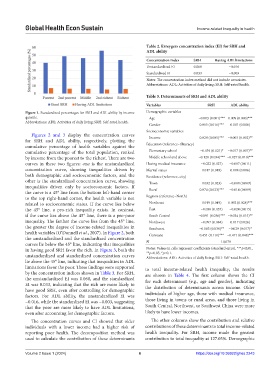
Figure 1. Standardized percentages for SRH and ADL ability by income Demographic variables
quintile. Age −0.003 (0.001)*** 0.009 (0.000)***
Abbreviations: ADL: Activities of daily living; SRH: Self-rated health.
Gender 0.065 (0.016)*** 0.001 (0.006)
Socioeconomic variables
Figures 2 and 3 display the concentration curves
for SRH and ADL ability, respectively, plotting the Income 0.028 (0.005)*** −0.005 (0.002)**
cumulative percentage of health variables against the Education (reference=illiteracy)
cumulative percentage of the total population, ranked Elementary school −0.039 (0.021)* −0.017 (0.007)**
by income from the poorest to the richest. There are two Middle school and above −0.128 (0.034)*** −0.027 (0.010)***
curves in these two figures: one is the unstandardized Having medical insurance −0.022 (0.027) −0.007 (0.011)
concentration curve, showing inequalities driven by Marital status 0.017 (0.018) 0.008 (0.006)
both demographic and socioeconomic factors, and the Residence (reference=city)
other is the standardized concentration curve, showing Town 0.032 (0.023) −0.008 (0.009)
inequalities driven only by socioeconomic factors. If
the curve is a 45° line from the bottom left-hand corner Rural 0.074 (0.023)*** −0.014 (0.009)
to the top right-hand corner, the health variable is not Regions (reference=North)
related to socioeconomic status. If the curve lies below Northeast 0.019 (0.049) 0.092 (0.028)***
the 45° line, a pro-rich inequality exists. In contrast, East −0.036 (0.035) −0.024 (0.015)
if the curve lies above the 45° line, there is a pro-poor South Central −0.091 (0.036)*** −0.034 (0.015)**
inequality. The farther the curve lies from the 45° line, Northwest −0.097 (0.084) 0.017 (0.026)
the greater the degree of income-related inequalities in Southwest −0.083 (0.039)** −0.029 (0.017)*
health variables (O’Donnell et al., 2007). In Figure 2, both Constant 0.451 (0.110)*** −0.471 (0.048)***
the unstandardized and the standardized concentration
curves lie below the 45° line, indicating that inequalities N 10,078
in having good SRH favor the rich. In Figure 3, both the Notes: Values in cells represent coefficients (standard error). ***p<0.01,
**p<0.05, *p<0.1.
unstandardized and standardized concentration curves Abbreviations: ADL: Activities of daily living; SRH: Self-rated health.
lie above the 45° line, indicating that inequalities in ADL
limitations favor the poor. These findings were supported to total income-related health inequality; the results
by the concentration indices shown in Table 3. For SRH, are shown in Table 4. The first column shows the CI
the unstandardized EI was 0.068, and the standardized for each determinant (e.g., age and gender), indicating
EI was 0.033, indicating that the rich are more likely to the distribution of determinants across income. Older
have good SRH, even after controlling for demographic
factors. For ADL ability, the unstandardized EI was individuals of higher age, those with medical insurance,
−0.016, while the standardized EI was −0.003, suggesting those living in towns or rural areas, and those living in
that the poor are more likely to have ADL limitations, South Central, Northwest, or Southwest China were more
even after accounting for demographic factors. likely to have lower incomes.
The concentration curves and CI showed that older The other columns show the contribution and relative
individuals with a lower income had a higher risk of contributions of these determinants to total income-related
reporting poor health. The decomposition method was health inequality. For SRH, income made the greatest
used to calculate the contribution of these determinants contribution to total inequality at 127.05%. Demographic

Volume 2 Issue 1 (2024) 6 https://doi.org/10.36922/ghes.2243