Page 17 - IJAMD-2-1

International Journal of AI for
Materials and Design
Predicting thermal conductivity of sintered Ag

A B

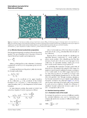
Figure 3. Comparison of microstructure finite element model before and after filling. (A) Schematic diagram of isolated islands in the model before air-
filling. (B) Schematic diagram of the model after air-filling. Green boxes indicate geometric model of sintered nano Ag. Blue boxes indicate pore regions of
sintered nano Ag. Red circles indicate isolated islands sintered nano Ag. Red dashed lines indicate the upper and lower boundary.
Abbreviations: T : Upper-temperature boundary condition; T : Lower temperature boundary condition.
u
b
2.1.2. Effective thermal conductivity computation where S is the total area of the finite element model, S i
For homogeneous materials, according to Fourier’s law of heat is the area of unit i, and q is the heat flux value of unit i in
yi
transfer, the rate of heat flow in the y-direction (1D form of the y-direction.
31
Fourier’s law of heat transfer) can be expressed as: Equation III is a discrete formula for calculating the
equivalent thermal conductivity k , which applies to
dT eq
q = − k d y (I) porous media models. After determining the heat flux
y
and area of each unit in the dense nano-Ag region in the
y-direction, the equivalent thermal conductivity of the
where q is the heat flow in the y-direction, k is thermal
y
conductivity, and dT/dy is the temperature gradient in the entire model can be obtained using Equation III.
y-direction. In calculating the equivalent thermal conductivity of
A simple modification of Equation I yields the formula sintered nano-Ag nanoparticles using the SEM images, the
for thermal conductivity: number of points n must be sufficient to ensure convergence
of the model results. In two SEM images obtained from
q y ( y − y b ) the same sintering process, 18 windows of 20 μm² were
u
k = − (II) extracted, and the number of pixels was 50 × 50, 100 × 100,
T − T b 150 × 150, and 200 × 200. Through simulation calculation,
u
where y is the coordinate of the upper boundary the thermal conductivity of each window under different
u
in the y-direction, y is the coordinate of the bottom extraction conditions was obtained (Figure 5A and B),
b
boundary in the y-direction, T is the temperature at the with the mean and range of thermal conductivity presented
u
upper boundary, and T is the temperature of the bottom for each extraction condition. Notably, the difference in
b
boundary. calculated thermal conductivity between a pixel size of
In finite element analysis, the model is divided into 150 × 150 and 200 × 200 is 3.3%.
units; thus, Equation II can be expressed as follows: 2.2. Machine learning method
n 2.2.1. Evaluation index of the model
q y ( y − y b )∑ S i
u
q y ( y − y b )S To evaluate the prediction accuracy of different models,
u
k eq = − = − i= 1 five statistical indicators were used to characterize and
)
)
(T − u TS (T − u TS compare the prediction accuracy of different data-driven
b
b
n models. 32-34
( y − y b )∑ qS
yi i
u
n
= − i= 1 (III) MSE = 1 ∑ (y − y *2 (IV)
)
)
(T − TS i n = 1 i i
u
b
Volume 2 Issue 1 (2025) 11 doi: 10.36922/ijamd.5744