Page 20 - IJAMD-2-1

International Journal of AI for
Materials and Design
Predicting thermal conductivity of sintered Ag

x
  x if >0 from the training samples should be equal to or close to
ReLU: fx (VII) the target value. The loss function is calculated as follows:
( ) = 
  θx if ≤x 0
1 l 2 1 l l− 1 l 2
( ,, , ) y =
An ANN with more hidden layers and neurons is J W b x 2 a − y = 2 2 σ (W a + b ) y− 2 (X)
typically regarded as a deep neural network (DNN).
1
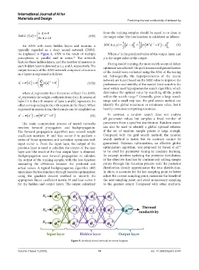
As displayed in Figure 8, ANN is the result of multiple Where a is the predicted value of the output layer, and
perceptrons in parallel and in series. The network y is the target value of the output.
36
features three hidden layers, and the number of neurons in During model training, the most widely accepted Adam
each hidden layer is denoted as i, j, and k, respectively. The optimizer was selected. The performance and generalization
output formula of the ANN network composed of neurons of the model were evaluated using the MSE of the testing
in n layers is expressed as follows:
set. Subsequently, the hyperparameters of the neural
 n  network are tuned based on the MSE value to improve the
l
a = σ ( ) σ i l ω ij l a l− 1 + b i ∑ l (VIII) performance and stability of the model. Grid search is the
z = 
i
j
 j= 1  most widely used hyperparameter search algorithm, which
where a represents the i-th neuron of layer l in ANN; determines the optimal value by searching all the points
l
i
37
w represents the weight coefficient from the j-th neuron of within the search range. Generally, given a large search
l
ij
layer l-1 to the i-th neuron of layer l; and b represents the range and a small step size, the grid search method can
l
i
offset corresponding to the i-th neuron in the l layer. When identify the global maximum or minimum value, but it
expressed in matrix form, the formula can be simplified as: heavily consumes computing resources.
l
a = σ ( ) σ z l = (W a l− 1 + b l ) (IX) In contrast, a random search does not analyze
l
all parameter values but samples a fixed number of
The main computation process of neural networks parameters from a specified distribution. Random search
involves forward propagation and backpropagation. can also be used to identify a global optimal solution
The forward propagation algorithm uses several weight if the set of random sample points is large enough.
coefficient matrices W and bias vector b to perform a Compared with the grid search method, the random
series of linear operations and activation operations with search method is faster, but its accuracy cannot be
input vector x. From the input layer, the output of the guaranteed. Bayesian optimization, an effective global
38
previous layer is used to calculate the output of the next optimization algorithm, was proposed by Snoek et al.
layer until the result of the final output layer is obtained. to be used for parameter tuning in machine learning.
Backpropagation uses forward propagation to calculate Its concept involves updating the posterior distribution
the output of the training sample, with the loss function of the objective function by continuously adding sample
measuring the difference between the predicted and points through the Gaussian process until the posterior
actual values. A typical backpropagation algorithm (BP) distribution closely approximates the true distribution.
minimizes the loss function through iterative optimization In short, it accounts for the last sampling point to better
using the gradient descent method to identify the adjust the current sampling point, maximize the benefit of
appropriate linear coefficient matrix W and bias vector b the next sampling point, and avoid unnecessary sampling
for the hidden and output layers. The output calculated to the greatest extent. Compared with other methods,

Figure 8. Artificial neural network structure diagram

Volume 2 Issue 1 (2025) 14 doi: 10.36922/ijamd.5744