Page 61 - IJB-10-1

International Journal of Bioprinting Microfluidic-assisted 3D bioprinting

proportional to the time so that there is laminar flow. For effective model whose parameters need to be calibrated
the sake of clarity, the quantities σ and ϵ are second-order with experimental data, e.g., acquired with a conical
tensors, while M is a fourth-order one. Here, we refer only rheometer (Figure 3b).
to shear stress, thus all three quantities are scalar, and the Although the HB constitutive law should be generalized
involved modulus is the shear modulus G.
in the appropriate tensor form to describe a generic flow,
Based on the aforementioned phenomenology, a the simpler Equation I will suffice here for an introductory
reliable rheological model of flowing biomaterial inks illustration of two configurations relevant to biofabrication.
should combine at least two ingredients, which are: Firstly, we consider the flow in a long capillary of radius R
0
i) the yield stress, like in a Bingham fluid, which: under a prescribed pressure gradient dp/dz| . Momentum
0
conservation
• is rigid (γ˙ = 0) if σ ≤ σ . Without loss of generality,
0
we assume hereafter that the stress is applied in 1 dr( ) dp ()II (II)
the positive direction, and therefore, σ is a positive r dr dz 0
quantity.
demands the force balance σ (r) = 1/2 dp/dz| r, where
0
• flows with a viscous stress/shear characteristic σ = the integration constant vanishes. From the latter, it is
σ + ηγ˙ if the yield stress is exceeded. clear that the shear stress tends to zero, approaching the
0
ii) a shear-thinning response, like in a power-law fluid, capillary axis. This shows that around the axis, r ≤ R = 2
p
with effective viscosity decreasing with the shear rate: σ /dp/dz| r, a solid region moving rigidly, the rigid plug,
0
0
σ = η˜(γ˙)γ˙, where η˜(γ˙) is the effective viscosity which should form since the yield stress is not exceeded. From the
in turn is expressed as ῆ(γ˙) = Kγ˙ . Here, K is called stress, using Equation I and γ˙ = du/dr, the velocity profile
n-1
the consistency index (units in the SI Pa . s ) and n in the capillary can be obtained as:
n
is the power-law exponent (n < 1). This combined n1
behavior is well described by the Herschel–Bulkley n 1 dp n / 1 R ( 0 R ) n r R p (III)
p

(HB) model, which for a simple shear flow reads: ur() n 1 2 K dz n1 n1 (III )
105

r
rR ))
0
R ( 0 R ) n ( P n R R 0 ,
p
P
0,

()I
 1/n 0 (I) which describes a rigid plug for r ≤ R and a shear thinning
p
K
[( 0 )/ ], 0 plug (n < 1) in the external part of the capillary (Figure 4a).
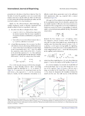
If n < 1, the viscosity decreases with the shear strength, As a second example, we consider the sheath flow of
leading to shear thinning behavior (shear thickening a Newtonian fluid used to focus the biomaterial in the
response would be obtained for n > 1), as shown in core of the capillary. Figure 4b shows a HB core and a
Figure 3a. To summarize, the model parameters are the plug, surrounded by the sheath flow in the annulus R ≤
0
yield stress σ , the exponent n < 1, and the consistency r ≤ R , where R demarcates the boundary between the
1
0
1
index K. Clearly, the HB constitutive relationship is an sheath and the core. The wall viscosity of the HB fluid

Figure 3.(a) Stress/shear characteristics, σ vs γ˙, of an HB fluid. The yield stress is set to σ = 0.25σw, where σ is the wall shear stress and η New is the reference
w
0
viscosity of a Newtonian fluid.In the inset, the effective viscosity η vs γ˙. (b) Working principle of a conical rheometer. The cone (axial section in red)
E f f
rotates with angular velocity ω with respect to the base (dark blue). The fluid velocity goes linearly from zero at the base to ωr at the rotating cone, hence
the shear is constant γ˙ = ω/tan(α).
Volume 10 Issue 1 (2024) 53 https://doi.org/10.36922/ijb.1404