Page 345 - IJB-9-4

International Journal of Bioprinting Bioprinting with machine learning

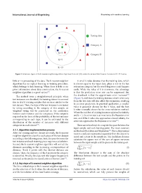
Figure 3. Schematic figure of the k-nearest neighbor algorithm. Reprinted from ref. [32] under the terms of the Creative Commons CC-BY license.

little or no processing of the data. The k-nearest neighbor A small k value denotes that the training data, which
algorithm has no explicit learning or training procedure, is almost equal to the input data, plays a role in the last
which belongs to lazy learning. When there is little or no estimation category, but the overfitting issue could happen
prior information about data construction, the k-nearest easily. While the value of k is enormous, the advantage
[29]
neighbor algorithm is a good option . is that the prediction error rate can be suppressed. But
[32]
the drawback is that the approximate error increases
The method owns a straightforward principle: when
test instances are classified, the training dataset is scanned (Figure 3), and then the training instance which is far away
from the test data will also affect the estimation, resulting
first to find k training samples that are most similar to the in an error prediction. In practical application, a smaller
test dataset. Then, the type of the test instance is evaluated value is generally chosen for the k value, and the best
by voting according to the category of this sample, or k value is usually chosen by the cross-validation method.
weighted voting will be conducted on the correlation When the number of training instances approaches infinity
between each instance and the test pieces. If the output is and k = 1, the error rate is at most twice the Bayesian error
required in the form of the probability of the test instance rate, and if the k value also approaches almost infinity, the
corresponding to each type, it can be estimated by the error rate approaches the Bayesian error rate .
[33]
distribution of the number of instances with different
categories in each dataset . There are several ways to compute the space between the
[30]
input sample and each training point. The most common
3.1.1. Algorithm implementation process methods are Euclidean and Manhattan . The n-dimensional
[34]
After the training and test dataset are ready, the k-nearest vectors x and y are represented separately from the data to be
neighbor algorithm classifies each piece of the test dataset tested and a point in the sample set. The Euclidean distance
according to the following steps. First, the space between the calculates the square root of the sum of square variances
test instance and each training piece requires a calculation. between the input sample and the pieces in the training set:
Second, the k-nearest neighbor algorithm will sort all the
i
distances according to the increasing correspondence of n x 2 (I)
y
distance. Third, k points with the shortest distance are i 1 i
chosen. Then, the frequency of the k points in the category The Manhattan distance is the sum of the absolute
is identified. Finally, the class with the largest frequency is difference between the test sample and the points in the
returned as the predictive classification of the test data . training set:
[31]
3.1.2. Key steps of k-nearest neighbor algorithm n x y (II)
i
i
The three critical steps in the k-nearest neighbor algorithm i1
are the selection of the k value, the calculation of distance, Before the calculation, the value of each feature should
and the formulation of the classification strategy. be normalized, which can help prevent the weights of

Volume 9 Issue 4 (2023) 337 https://doi.org/10.18063/ijb.739