Page 22 - IJB-9-6

International Journal of Bioprinting CFD analysis for multimaterial bioprinting conditions

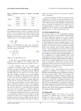
Table 1. Rheological parameters of alginate and gelatin solution was achieved when these parameters reached a
solutions [34,42] state of convergence.
Content n k [Pa s ] To further investigate the effect of nozzle geometries
n
Alginate 0.5 w/v% 0.977 0.032 (cylindrical and conical) and process parameters on cell
1.0 w/v% 0.895 0.119 viability, the flow rate, velocity magnitude, and shear stresses
1.5 w/v% 0.840 0.346 at the outlet, as well the axial discharge of the dispensing
pressure along the printing head, were evaluated for the
Gelatin 7.0 w/v% 0.795 0.240 converged solution. A variety of nozzle outlet diameters,
ranging from 0.25 to 2.00 mm, were examined at different
Materials to be printed through pneumatic (compressed inlet pressures (0.1–3.0 bar) for both nozzle types.
air), mechanical (piston or screw), or solenoid (electrical 2.2. Mesh independence test
pulses) driven printheads must exhibit shear-thinning The 3D flow domain of the KSM-integrated printing
properties, as this behavior allows to reduce shear stresses heads was discretized, using the selective meshing feature
during the printing process and to enhance cell viability. of ANSYS Workbench meshing tool to create as many
−1
The shear rate γ˙(s ) can be defined as follows:
structured (hexahedral) elements as possible, and fill the
du P remaining parts with tetrahedron elements. In this case,
 r (V) as the printing head consists of multiple bodies, we used
dr 2 L the patch conforming method for the Y-shaped main body
where r (m) is the radius of the pipe, L (m). According to including the KSM, and the sweep method for sweepable
Metzner et al. , the generalized Reynolds number for a bodies, such as barrels, and the other cylindrical parts
[41]
shear-thinning fluid is given by: (Figure 1). The mesh quality was refined near the mixing
u 2 n D n elements, and inflation layers were created for the pipe walls,
Re n (VI) to capture the flow fields more precisely in those places. To
2
k n6 obtain reliable numerical results, grid-independence tests
8 n were conducted for all needle geometries with varying
outlet diameters. These preliminary test results enabled to
where D is the pipe diameter (m). establish the best node layout and cell density, for numerical
In this study, non-crosslinked alginate and gelatin accuracy and computational load. Thus, a mesh sensitivity
solutions were selected as the working fluids. The study was performed to observe how the outlet velocity
rheological data for both materials arepresented in Table 1. magnitude deviates as the number of grids increased. The
discretization of the models used in CFD simulations for
In the simulations, all solid boundaries were
considered as stationary walls, where the “nonslip” both nozzle types is shown in Figure 1.
boundary condition was applied. Moreover, by adjusting As shown in Figure 2, the calculated maximum velocity
the dispensing pressure at the inlet boundaries, different magnitude was stabilized by increasing the number of
Reynolds numbers were obtained for the flow domain. elements. Grid independence was achieved for the cylindrical
The outlet boundary condition was set as atmospheric and conical nozzle models, with 6 × 10 elements and
5
pressure in all simulations. The stationary solver was used 8 × 10 , respectively, beyond that no substantial changes were
5
to resolve the model, and calculations were carried out observed. Based on these preliminary convergence test results,
using pressure–velocity coupling (Coupled algorithm). a mesh of 7.3 × 10 and 9.8 × 10 elements were chosen as the
5
5
To discretize the momentum and pressure formulation, a optimal mesh density, as it provides high accuracy of results
second-order upwind method was used, while the least- with a shorter computational time required for convergence.
squares cell-based method was used for the gradients. The maximum skewness for all model meshes were lower than
The relaxation parameters for pressure and momentum 0.85, with a minimum value of 2.3 × 10 and a minimum
−5
were set as 0.5 and set to 1.0, for body forces and density, element quality of 0.09, which according to the literature is a
respectively. For all simulations, the relative residuals of nice evidence of good mesh quality .
[43]
the velocity and continuity components were less than
10 , after approximately 1000 iterations, corresponding to 2.3. Mixing index
−5
a reasonably short calculation time (≤30 min) on an Intel The distributive capacity of the Kenics mixer was also
processor with four cores. Convergence analysis was also investigated for different flow velocities. Distributive
tested, by monitoring the area-weighted average values of mixing, also known as simple or extensive mixing,
the shear stress and the velocity at the outlet. A stationary represents the spatial distribution of the components

Volume 9 Issue 6 (2023) 14 https://doi.org/10.36922/ijb.0219