Page 136 - IJOCTA-15-1

R. Bagri, G. Sachdev, D. Agarwal / IJOCTA, Vol.15, No.1, pp.123-136 (2025)

(a) (b)

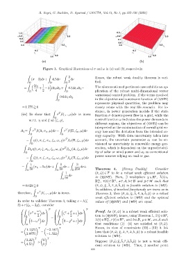
Figure 1. Graphical illustrations of σ and ω in (a) and (b), respectively.

Z Z Z
3 Hence, the robust weak duality theorem is veri-
= (σ−3)dν + 4.5dν − dν
Ω Ω Ω 5 fied.
Z Z

3t 1 1
= + −3 dt 1 dt 2 + 4.5dt 1 dt 2 − The aforementioned pertinent case exhibits an ap-
Ω 4 2 Ω plication of the robust multi-dimensional vector
Z
variational control problem. If the terms involved
0.6dt 1 dt 2
Ω in the objective and constraint function of (UVP1)
represents physical quantities, the problem may
=1.775≧0 closely relate with the real life scenario. For in-
stance, in power generation models if the state
Z
T
(iii) To show that τ β(., ., µ)dν is invex function σ denotes power flow in a grid, while the
Ω
w.r.t. η and ξ at (ζ, ϱ), control function ω indicates the power demands in
different regions, the objectives of (UVP1) can be
interpreted as the minimization of overall grid en-
Z Z
T
T
A 4 = τ β(Λ, σ κ , µ)dν − τ β(Π, ζ κ , µ)dν ergy loss and the deviation from the intended en-
Ω Ω
ergy capacity. With data uncertainty taken into
Z
T
− η(t, σ, ζ, σ κ , ζ κ , ω, ϱ)τ β σ (Π, ζ κ , µ)dν account, the uncertain parameter a 1 can be en-
Ω visioned as uncertainty in renewable energy gen-
Z
T
− D κ η(t, σ, ζ, σ κ , ζ κ , ω, ϱ)τ β σ κ (Π, ζ κ µ)dν eration, which is dependent on the unpredictabil-
Ω ity of solar or wind power and a 2 as conventional
Z
T
− ξ(t, σ, ζ, σ κ , ζ κ , ω, ϱ)τ β ω (Π, ζ κ , µ)dν power sources relying on coal or gas.
Ω
Z Z Z
1 1 3
= (σ t 1 −5ω)dν + dν − dν+
Ω 50 Ω 50 Ω 250 Theorem 4. [Strong Duality] Consider
Z
1 (¯σ, ¯ω)∈T to be a robust weak efficient solution
dν p ¯
50 to (RUVP). Then, ∃ multipliers ¯χ∈R , λ(t)∈
Ω
¯
m
n
R , ¯τ(t)∈R , ¯ a ∈A, b∈B and ¯µ∈M such that
+
¯
¯
=0.028≧0 (¯σ, ¯ω, ¯χ, λ, ¯τ, ¯ a, b, ¯µ) is feasible solution to (WD).
In addition, if involved functionals are invex as in
Z
T
¯
¯
therefore, τ β(., ., µ)dν is invex. Theorem 3, then (¯σ, ¯ω, ¯χ, λ, ¯τ, ¯ a, b, ¯µ) is a robust
Ω
weak efficient solution to (WD) and the optimal
In order to validate Theorem 3, taking ε=λ(ζ − values of (RUVP) and (WD) are equal.
−3ϱ), consider
3)+τ(ζ t 1
 
Z T Z T
ω ϱ Proof. As (¯σ, ¯ω) is a robust weak efficient solu-
2
2
σ + dν ζ + +ε dν
p
 Ω  −  Ω 
 2   2  tion to (RUVP), hence, using Theorem 1, ∃ ¯χ∈R ,
Z
Z
¯ m n ¯
 2   2  λ(t)∈R , ¯τ(t)∈R , and b∈B, ¯µ∈M , ¯ a ∈A such
3−ω dν 3−ϱ +ε dν +
△ △ that conditions (1)−(4) are satisfied at (¯σ, ¯ω).
T T Hence, in view of constraints (10)−(13) it fol-
1.1375 −2.187
¯
¯
= − lows that (¯σ, ¯ω, ¯χ, λ, ¯τ, ¯ a, b, ¯µ) is a robust feasible
2.9775 −1.552
solution to (WD).
T T
3.32 0 ¯ ¯
= > . Suppose (¯σ, ¯ω, ¯χ,λ,¯τ,¯ a,b, ¯µ) is not a weak effi-
4.53 0
cient solution to (WD). Thus, ∃ another point
130