Page 24 - IJOCTA-15-1

S. Karahan Orak, N. Aydin, E. Karatas / IJOCTA, Vol.15, No.1, pp.14-24 (2025)

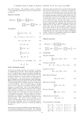
the initial inventory. This equality is given in equation equals the previous month’s stock and the month’s produc-
8. Non-negativity constraints are given in equation 9 and tion minus the sales amount. The demand constraint en-
equation 10. sures that the sales amount and the unmet demand equal
the total demand. The safety stock constraint ensures that
Objective Function the company maintains at least the safety stock level. Af-
ter obtaining the amount to be stocked, the box constraint
T I T I calculates the number of boxes required, and the ware-
X X X X
Minimizez = y iU it + D iR it− house constraint ensures that the total number of boxes
t=1 i=1 t=1 i=1 does not exceed warehouse capacity. The initial stock con-
T I T I straint is added since the company starts production with
X X X X
c iN it + h iL it (1) safety stock in the first month. In stochastic models, de-
t=1 i=1 t=1 i=1 cisions made in the first stage should be consistent across
all scenarios, known as the non-anticipativity constraint.
Constraints This constraint ensures that the production quantities de-
termined in the first stage remain the same in subsequent
I
X months. Finally, the non-negativity constraint is added to
a ijU it ≤ F jG j ∀j, t (2)
ensure all decision variables are positive.
i=1
R it − U it = R i(t−1) − N it ∀i, t ≥ 1 (3)
Objective Function
N it + L it = E it ∀i, t (4)
S T I
X X X
R it ≥ B i ∀i, t (5) Minimize z = P s D iR its−
s=1 t=1 i=1
!
T I T I T I
R it X X X X X X
≤ K it ∀i, t (6) c iN its + y iX its + h iL its (11)
W i
t=1 i=1 t=1 i=1 t=1 i=1
I
X
K it ≤ Q ∀t (7) Constraints
i=1
Capacity Constraint
R i0 = B i ∀i (8) I
X
a ijX its ≤ F jG j ∀j, t, s (12)
R it, L it, N it, U it ≥ 0 and integer ∀i, t (9) i=1
Inventory Constraint
K it ≥ 0 ∀i, t (10)
R its − X its = R i(t−1)s − N its ∀i, t, s (13)
3.2.2. Stochastic model
Demand Constraint
In modern production systems, the presence of stochas-
tic parameters is inevitable. These stochastic parameters N its + L its = E its ∀i, t, s (14)
can be considered when solving real systems through sto-
chastic modeling. The stochastic model developed for the Safety Stock Constraint
production planning of a factory with uncertain demands
is outlined below. The system aims to be optimized us-
R its ≥ B i ∀i, t, s (15)
ing the Sample Average Approximation (SAA) algorithm.
With its scenario-based structure, the SAA method offers
a holistic perspective for assessing numerous conditions in Warehouse Constraint
I
real-world problems. Due to its rapid response capabil- X
ity, it can solve large-scale problems involving extensive K its ≤ Q ∀t, s (16)
scenarios in a short time. One of the main reasons for i=1
preferring SAA in the production planning of the company Storage Constraint
that manufactures clamps is to present to the decision-
maker how the result will change in possible situations by R its ≤ K its ∀i, t, s (17)
creating different scenarios. Here, the impact of stochastic W i
parameters is considered in creating scenarios and solv-
ing via the SAA method, supporting the approach to the Initial Inventory Constraint
optimal solution. The model becomes stochastic and is R i0s = B i ∀i, s (18)
solved by incorporating scenario effects into the objective
function and constraints. As in the deterministic model,
Non-anticipativity Constraints
the stochastic objective function is initially provided by
Equation 11. ′ ′
X its = X its ′ t = 1, s = 1, ∀i, s | s < s (19)
′
The capacity constraint is included to ensure that daily ma- N its = N its ′ t = 1, s = 1, ∀i, s | s < s ′ (20)
′
chine working capacities are not exceeded. The inventory L its = L its ′ t = 1, s = 1, ∀i, s | s < s ′ (21)
′ ′
constraint ensures that the inventory amount for the month R its = R its ′ t = 1, s = 1, ∀i, s | s < s (22)
18