Page 25 - IJOCTA-15-1

Significance of stochastic programming in addressing production planning under uncertain demand...

′
K its = K its ′ t = 1, s = 1, ∀i, s | s < s ′ (23) Objective Function z= -4.696.619TL
Non-negativity Constraints As Table 1 indicates, the model has determined the opti-
mal production quantities: 22.210 for Product 1, 32.190 for
X its, R its, L its, N its ≥ 0 and integer Product 2, and 18.597 for Product 3. Considering these
∀i, t, s (24) quantities, the model aims to minimize costs while con-
sidering unmet demand and inventory levels. The model
K its ≥ 0 ∀i, t, s (25)
views the sales loss for Product 3 as advantageous in align-
ment with its minimization objective.
3.3. SAA application
However, when the stochastic model was solved by consid-
In the application of SAA, the product sales table was ini- ering the randomness of demand beyond the expected value
tially considered in scenario generation to create the first and assuming an infinite number of possible demands be-
step of the SAA application. Considering the minimum tween the minimum and maximum sales values within the
and maximum values of products with one year of sales annual data, the best solutions ranged between 4 million
data, it was assumed that an infinite number of orders and 5 million. The model calculated the required produc-
could be received within this range. This assumption al- tion quantity for each month, the amount to be sold, and
lowed the integration of the uncertainty and randomness the consequent sales loss, i.e., the unmet demand. Pro-
of future demands into the model by generating random duction quantities were determined for each month and
demand quantities over 6 months between the minimum scenario, resulting in varying sales, production, and inven-
and maximum values. Clusters were formed to account tory values according to the changing demand quantities.
for scenario variability, and the model’s best result was
calculated. A sample pool consisting of 10 clusters was
created in total. In the first phase of the SAA application, optimal solu-
tion results were obtained for the relevant clusters within
different scenarios.
In each cluster, cases with five and ten scenarios were mod-
eled, respectively. Within these scenarios, the objective These results were subsequently subjected to performance
function value of each cluster and the optimal produc- testing within a large sample. During the testing phase,
tion quantity required in the first phase were obtained. the initial production quantities that the factory needed to
A test sample with 500 scenarios was created to evalu- produce in the first month were provided to the model as
ate the model’s performance. The production quantities parameters, and the success of the first-stage decision vari-
obtained were tested in the large sample. If the values ables obtained under stochastic conditions was evaluated
obtained are acceptable to the decision-maker, one of the within a large sample. The production quantities obtained
values determined within the appropriate cluster can be for each product in each cluster solution were taken as the
selected for implementation. If better results are desired, first-stage values within the large sample for performance
changes can be made to the sample and scenario number evaluations. The values obtained were sequentially pro-
to achieve better outcomes. For this study, two different vided to the model created for the test sample, and the
scenario quantities were applied sequentially, and the re- result of the objective function was calculated. The gap
sults were obtained. The largest scenario was accepted as value was obtained by calculating the difference between
10 scenarios for each cluster. the objective function value obtained from the cluster so-
lutions and the objective function value of the large sample.
3.4. Results The mean and standard deviation values of the obtained
objective function and gap values were compared to make
The potential demand quantity was calculated within the comparisons.
expected value framework by considering the annual sales
data, and the deterministic model was solved based on As seen in Table 2, m represents the number of clusters,
these values. In the cost minimization model, the objec- while Product 1, Product 2, and Product 3 show the first-
tive function value was determined as z min = −4.696.619. stage decision variable values that the products should take
This value is the output of the objective function, assuming within the cluster. The optimal solution value of the model
that demand each month matches the expected value with- is expressed as z. The value of the objective function ob-
out considering stochastic variations. The model assumes tained by testing the first-stage decision variables within
the same production quantities for the remaining months the large sample is denoted by Z. The difference between
of the year, aside from the initial month’s production, by these two objective function values represents the gap.
evaluating the situation at time t to provide the production
In the initial phase, small samples were created as part of
quantities that will yield the minimum cost. Fluctuations
the SAA algorithm’s implementation steps, and the model
in demand were not considered, and the model provided a
was solved, calculating decision variables and the objective
solution based on the current evaluation of which product
function. Table 2 shows the optimal solution values when
group had high demand, deeming it profitable.
10 clusters were created, each containing 5 scenarios with
randomly obtained demand quantities.
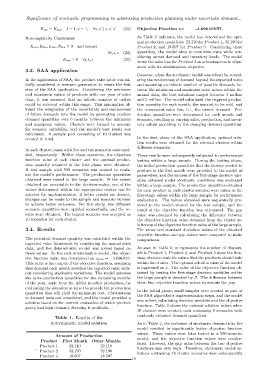
Table 1. Results of the
deterministic model solution As in Table 2, the inclusion of stochastic demand into the
model resulted in significantly better objective function
values. These values were later tested in a 500-scenario
Amount of Production
model, and the objective function values were recalcu-
Product First Month Other Months
lated. However, the gap value between the two objective
Product 1 22.110 22.110
, functions was very high. Therefore, stochastic model so-
Product 2 32.190 32.190
lutions containing 10 cluster scenarios were subsequently
Product 3 18.597 18.597
19