Page 26 - IJOCTA-15-1

S. Karahan Orak, N. Aydin, E. Karatas / IJOCTA, Vol.15, No.1, pp.14-24 (2025)

Table 2. Monte Carlo Simulation N=5, m=10
Cluster No Product Product Product Value of Test Gap
1 2 3 Objective result in
Function large
(z) sample
(Z)
1 23.098 30.341 20.810 -5.001.679 -5.019.889 18.209,91
2 20.970 29.681 22.461 -4.992.230 -5.019.852 27.621,80
3 22.193 30.090 21.512 -4.896.529 -5.019.885 123.355,77
4 20.675 34.577 22.690 -4.754.399 -5.020.083 265.683,96
5 20.862 34.945 22.545 -5.054.492 -5.020.103 -34.389,43
6 23.865 29.741 20.215 -5.039.257 -5.019.855 -19.402,07
7 23.687 35.231 20.353 -5.259.730 -5.020.119 -239.610,99
8 20.278 34.669 22.998 -4.936.899 -5.020.083 83.184,23
9 20.898 34.999 22.517 -4.954.620 -5.020.106 65.485,57
10 20.889 32.499 22.524 -5.048.848 -5.019.986 -28.861,94

performed.

As in Table 3 , increasing the number of scenarios within
the clusters reduces the difference between z and Z. This
result is displayed in the gap column. It is observed that
increasing the number of scenarios improves the perfor-
mance of the z values obtained within the large sample.

As a result, the summary table named Table 4 was ob-
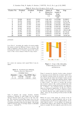
tained. Figure 1. Graph of the relationship
between objective function values
and deviations
Table 4. The Relationship Between
Objective Function Values and
Deviation Values
Figure 1 presents the objective function values obtained
Scenarios z avg Z avg=N’500 Z Dev by analyzing scenarios within the stochastic model. Here,
N = 5 -4.993.868 -5.019.996 115 two objective function values are provided: One derived
N = 10 -4.977.221 -5.020.004 92,98 from solving the set within the stochastic model, and the
other obtained from solving the resulting solution values
within a large sample. Scenario-based solutions are given
in Table 2 and 3. The aim is to calculate the averages
and deviation values of the z-values obtained from each
set’s solution and the z-values derived from the large sam-
ple. In Figure 1, the calculated average and deviation
values are summarized graphically. As observed in Figure
1, increasing the number of scenarios positively impacts
the objective function value while reducing the deviation
values. Thus, the set providing the best solution should
be selected.
Table 4 presents the average objective function
values(z avg) obtained for each cluster and the average
objective function values (Z avg) tested in the large sam- Within the scope of this study, the outputs of the 10-
ple. The deviations from the large sample (Z dev) are also scenario model were deemed sufficient, and one of the
calculated. The deviation value decreases as the number successful clusters was selected for implementation. In the
of scenarios increases within the test sample. The average table (Table 4) with N = 10, the cluster to be chosen can
objective function value of the large sample is calculated be determined based on the criterion the decision-maker
as z min = −5.020.004 TL. wishes to consider. For this study, the point with the best
20