Page 45 - IJOCTA-15-2

M. M. Parsa, K. Sayevand, H. Jafari, I. Masti / IJOCTA, Vol.15, No.2, pp.225-244 (2025)

β = 0.4 β = 0.5 β = 0.6
1 1 1
0.8 0.8 0.8
v(s,τ) 0.6 v(s,τ) 0.6 0.4 v(s,τ) 0.6
0.4
0.4
0.2 0.2 0.2
0 0 0
1 1 1
1 1 1
0.8 0.8 0.8
0.5 0.6 0.5 0.6 0.5 0.6
0.4 0.4 0.4
0.2 0.2 0.2
τ 0 0 s τ 0 0 s τ 0 0 s
β = 0.7
1
0.8
v(s,τ) 0.6 0.4
0.2
0
1
1
0.8
0.5 0.6
0.4
0.2
τ 0 0 s
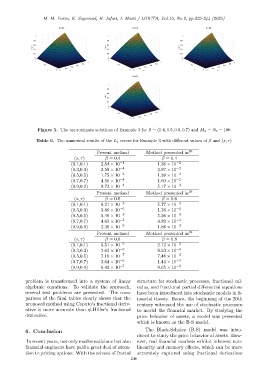
Figure 5. The approximate solutions of Example 3 for β = (0.4, 0.5, 0.6, 0.7) and M x = N t = 100
Table 6. The numerical results of the L 1 errors for Example 3 with different values of β and (s, τ)

Present method Method presented in 39
(s, τ) β = 0.4 β = 0.4
(0.1,0.1) 2.84 × 10 −4 1.36 × 10 −2
(0.3,0.3) 3.59 × 10 −4 2.97 × 10 −2
(0.5,0.5) 1.75 × 10 −3 1.38 × 10 −3
(0.7,0.7) 4.56 × 10 −4 1.60 × 10 −2
(0.9,0.9) 9.72 × 10 −4 5.17 × 10 −3
Present method Method presented in 39
(s, τ) β = 0.6 β = 0.6
(0.1,0.1) 6.21 × 10 −5 5.77 × 10 −3
(0.3,0.3) 3.86 × 10 −6 1.76 × 10 −2
(0.5,0.5) 5.46 × 10 −5 5.56 × 10 −3
(0.7,0.7) 4.63 × 10 −5 4.89 × 10 −3
(0.9,0.9) 2.36 × 10 −6 1.86 × 10 −3
Present method Method presented in 39
(s, τ) β = 0.8 β = 0.8
(0.1,0.1) 5.51 × 10 −6 2.12 × 10 −3
(0.3,0.3) 7.63 × 10 −6 9.53 × 10 −3
(0.5,0.5) 7.16 × 10 −7 7.46 × 10 −3
(0.7,0.7) 3.64 × 10 −6 1.44 × 10 −3
(0.9,0.9) 6.43 × 10 −7 9.65 × 10 −3

problem is transformed into a system of linear structure for stochastic processes, fractional cal-
algebraic equations. To validate the approach, culus, and fractional partial differential equations
several test problems are presented. The com- have been introduced into stochastic models in fi-
parison of the final tables clearly shows that the nancial theory. Hence, the beginning of the 20th
proposed method using Caputo’s fractional deriv- century witnessed the use of stochastic processes
ative is more accurate than ψ-Hilfer’s fractional to model the financial market. By studying the
derivative. price behavior of assets, a model was presented
which is known as the B-S model.
6. Conclusion The Black-Scholes (B-S) model was intro-
duced to study the price behavior of assets. How-
In recent years, not only mathematicians but also ever, real financial markets exhibit inherent non-
financial engineers have paid a great deal of atten- linearity and memory effects, which can be more
tion to pricing options. With the advent of fractal accurately captured using fractional derivatives
240