Page 43 - IJOCTA-15-2

M. M. Parsa, K. Sayevand, H. Jafari, I. Masti / IJOCTA, Vol.15, No.2, pp.225-244 (2025)
Table 1. The maximum numerical errors and computational orders of Example 1 where
M x = 100 and different N t and β values

N t β = 0.1 Order β = 0.5 Order β = 0.9 Order
32 3.5436 × 10 −3 - 4.7725 × 10 −4 - 8.4154 × 10 −5 -
64 7.3850 × 10 −3 1.32 7.1826 × 10 −5 1.38 1.9827 × 10 −5 1.59
128 5.9453 × 10 −4 1.33 5.9920 × 10 −6 1.39 3.1951 × 10 −6 1.61
256 9.1414 × 10 −5 1.35 2.0114 × 10 −6 1.41 6.4299 × 10 −7 1.63
Table 2. The numerical results for Example 1 where β = 0.7 and M x = 100 and different
values of ∆t

Present method Method presented in 36
∆t L ∞ Order L ∞ Order
1 3.7264 × 10 −4 - 0.0037 -
10
1 2.1640 × 10 −5 1.43 0.0015 1.27
20
1 4.4052 × 10 −5 1.41 6.2714 × 10 −4 1.29
40
1 5.7631 × 10 −6 1.47 2.5377 × 10 −4 1.31
80
Table 3. The numerical results for Example 1 where β = 0.7 and M x = 150 and different
values of ∆t

Present method Method presented in 30
∆t L ∞ Order L ∞ Order
1 4.7641 × 10 −5 - 5.821 × 10 −3 -
10
1 8.9002 × 10 −5 1.48 2.304 × 10 −3 1.33
20
1 3.1383 × 10 −6 1.51 9.081 × 10 −4 1.34
40
1 9.5381 × 10 −7 1.52 3.572 × 10 −4 1.34
80

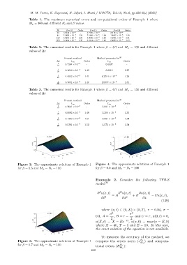
β = 0.5
1 1.5 β = 0.9
u(x,t) 0.5 u(x,t) 1
0 0.5
-0.5 0
1 1
1 1
0.5 0.6 0.8 0.5 0.6 0.8
0.4 0.4
0.2 0.2
0 0 0
t 0 x t x
Figure 2. The approximate solutions of Example 1 Figure 4. The approximate solutions of Example 1
for β = 0.5 and M x = N t = 100 for β = 0.9 and M x = N t = 100

Example 2. Consider the following TFB-S
model: 37

2
β
∂ u(x, t) ∂ u(x, t) ∂u(x, t)
= A + B − Cu(x, t),
∂t β ∂x 2 ∂x
(139)
where (x, t) ∈ (0, X) × (0, T), r = 0.04, σ =
0.6 β = 0.7 σ 2 σ 2
0.3, A = , B = r − and C = r, u(0, t) = 0,
u(x,t) 0.4 2 −rt 2
0.2 u(X, t) = X − Ee , u(x, 0) = max(x − E, 0)
where X = 40, T = 1 and E = 10. In this case,
0
1
1 the exact solution of the equation is not available.
0.8
0.5 0.6
0.4
0.2
t 0 0 x
To measure the accuracy of the method, we
Figure 3. The approximate solutions of Example 1 compute the errors norm (e N t ) and computa-
M x
for β = 0.7 and M x = N t = 100 tional orders (R N t ):
M x
238