Page 44 - IJOCTA-15-2

Analyzing the Black-Scholes equation with fractional coordinate derivatives using . . .
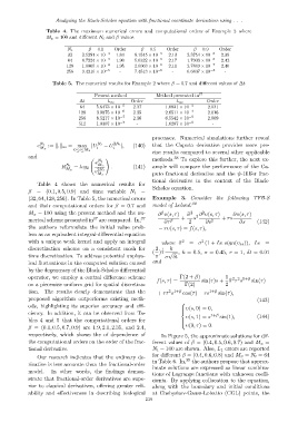
Table 4. The maximum numerical errors and computational orders of Example 2 where
M x = 100 and different N t and β values

N t β = 0.1 Order β = 0.5 Order β = 0.9 Order
32 2.5291 × 10 −3 1.84 8.1545 × 10 −5 2.13 2.3754 × 10 −6 2.39
64 8.7224 × 10 −4 1.90 5.6322 × 10 −5 2.17 1.7939 × 10 −6 2.42
128 1.0005 × 10 −4 1.95 2.6063 × 10 −5 2.11 2.7869 × 10 −7 2.40
256 9.4216 × 10 −5 - 7.4513 × 10 −6 - 6.6837 × 10 −8 -

Table 5. The numerical results for Example 2 where β = 0.7 and different values of ∆t

Present method Method presented in 37
∆t L ∞ Order L ∞ Order
64 5.6473 × 10 −5 2.37 1.0831 × 10 −3 2.031
128 3.9875 × 10 −6 2.35 2.6511 × 10 −4 2.016
256 8.5217 × 10 −7 2.36 6.5542 × 10 −5 2.009
512 1.0307 × 10 −7 - 1.6287 × 10 −5 -

processes. Numerical simulations further reveal
e N t := ∥.∥ ∞ = max |U N t − U 2N t |, (140) that the Caputo derivative provides more pre-
M x i i
0≤i≤M x
cise results compared to several other applicable
and 38
! methods. To explore this further, the next ex-
e N t
R N t = log 2 M x . (141) ample will compare the performance of the Ca-
M x 2N t
e
M x puto fractional derivative and the ψ-Hilfer frac-
tional derivative in the context of the Black-
Table 4 shows the numerical results for
Scholes equation.
β = (0.1, 0.5, 0.9) and time variable N t =
(32, 64, 128, 256). In Table 5, the numerical errors Example 3. Consider the following TFB-S
and their computational orders for β = 0.7 and model of Leland: 39
M x = 100 using the present method and the nu- ∂ υ(s, τ) b σ 2 2 ∂ υ(s, τ) ∂υ(s, τ)
2
β
merical scheme presented in 37 are compared. In, 37 ∂τ β + 2 s ∂s 2 + rs ∂s (142)
the authors reformulate the initial value prob- − rυ(s, τ) = f(s, τ),
lem as an equivalent integral-differential equation
with a unique weak kernel and apply an integral where bσ 2 = σ (1 + Le sign(υ ss )), Le =
2
discretization scheme on a consistent mesh for 2 1 k
( ) 2 √ , k = 0.5, σ = 0.45, r = 1, δt = 0.01
time discretization. To address potential unphys- π σ δt
ical fluctuations in the computed solution caused and
by the degeneracy of the Black-Scholes differential
operator, we employ a central difference scheme Γ(2 + β) 1 2 2 1+β
f(s, τ) = sin(τ)s + bσ τ s sin(τ)
on a piecewise uniform grid for spatial discretiza- Γ(2) 2
2 1+β
tion. The results clearly demonstrate that the + rτ s cos(τ) − rs 1+β sin(τ),
proposed algorithm outperforms existing meth- (143)

ods, highlighting its superior accuracy and effi-
υ(s, 0) = 0,

ciency. In addition, it can be observed from Ta- 
υ(s, 1) = s 1+β sin(1), (144)
bles 4 and 5 that the computational orders for 

 υ(0, τ) = 0.
β = (0.1, 0.5, 0.7, 0.9) are 1.9, 2.1, 2.35, and 2.4,
respectively, which shows the of dependence of In Figure 5, the approximate solutions for dif-
the computational orders on the order of the frac- ferent values of β = (0.4, 0.5, 0.6, 0.7) and M x =
tional derivative. N t = 100 are shown. Also, L 1 errors are reported
Our research indicates that the ordinary de- for different β = (0.4, 0.6, 0.8) and M x = N t = 64
in Table 6. In, 39 the authors propose that approx-
rivative is less accurate than the fractional-order
imate solutions are expressed as linear combina-
model. In other words, the findings demon-
tions of Lagrange functions with unknown coeffi-
strate that fractional-order derivatives are supe- cients. By applying collocation to the equation,
rior to classical derivatives, offering greater reli- along with the boundary and initial conditions
ability and effectiveness in describing biological at Chebyshev-Gauss-Lobatto (CGL) points, the
239