Page 76 - IJOCTA-15-2

Hybridizing biogeography-based optimization and integer programming for solving the travelling tournament ...

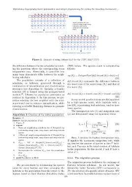
Figure 2. Example of using Relaxed ILP for the TTP( RILP-TTP)

the difference between the two schedules by count- (HSI) values. The species count is computed as
ing the positions where the corresponding team follows:
assignments vary. Essentially, it quantifies how
many team placements differ between the neigh-
sp (S i ) = IntegerPart [dif trcost (S i ) ∗ ln(i) ∗ i]
boring schedules.
(21)
The population consists of a collection of dif trcost (S i ) represents the difference between
schedules, or habitats, generated through a
the travel cost of the worst team (S 1 ) and that of
combination of intensification and diversification
the team (S i ).
strategies (see Algorithm 3). Initially, a feasible
schedule (S) is formed using the polygon-based
40
method, , followed by population generation as dif trcost (S i ) = travel cost (S 1 )−travel cost (S i )
(22)
outlined in Algorithm 3. In this process, we pri-
In our model, good solutions are distinguished
oritize selecting the best neighbor with the mini-
by a high species count, while habitats with a
mum travel cost to enhance intensification, while
low HSI, representing bad solutions, tend to have
ensuring a suitable Hamming distance to promote
diversification. fewer species.
The immigration rate (λ) and emigration rate
Algorithm 3 Creation of the initial population (µ) are determined using the equations below:
Require: S.
Ensure: Initial population (Pop) !
1: Pop ← S λ i = I sp i (23)
2: repeat 1 − P Pop−size
3: Form all neighboring schedules for S Neigh(S) by i=1 sp i
performing swap team, swap home and swap rounds sp i (24)
Pop−size
µ i = E × P
moves
i=1 sp i
4: //Form all neighboring schedules for S Neigh(S) by
performing swap team, swap home and swap rounds Here, I denotes the highest immigration rate,
moves . E signifies the maximum emigration rate, while
′ ′ ′
5: S best : ∀S ∈ Neigh(S), (travel cost(S best ) − th
′ ′ sp i denotes the number of species in the i habi-
distance hamming(S best , S)) < (travel cost(S ) − tat, and Pop-size is the total number of habitats
′
distance hamming(S , S))
′ in the population. In this model, I and E have a
6: Incorporates the solution S best into the population
Pop value of 1.
′
7: S ← S best
8: until Population is filled 3.2.4. The migration process
The migration process facilitates the exchange of
The process starts by determining the species features between solutions. In our model, the
count for every habitat and then arranging the Suitability Index Variable (SIV) corresponds to
habitats in the population from the lowest to the Ft: the schedule of a specific subset of teams. SIV
highest based on their Habitat Suitability Index attributes from favorable habitats replace those of
271