
Page 73 - IJOCTA-15-2
P. 73
M. Khelifa et. al. / IJOCTA, Vol.15, No.2, pp.264-280 (2025)
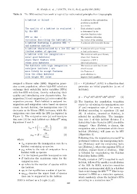
Table 3. The BBO method framework is inspired by mathematical principles from biogeography
A habitat or Island → A solution to the optimization
problem is modeled
as a vector
The quality of a habitat is evaluated → Each solution’s quality
by the HSI is determined by its
objective function value
SIV or the → The variables defending
variables describing the habitability the vector of the solution
A habitat featuring a greater HSI → A solution with favorable fitness
and numerous species
A habitat characterized by a low HSI and → A solution with poor fitness
limited number of species or bad performance
A habitat with low immigration→ The solutions with good fitness,
rate( good habitats) share their Features
share their feature with (migration of SIV )
other poor habitats with bad solutions
The habitats with high immigration → The solutions with bad fitness
rate(poor habitats ) are should accept
more likely to accept features the Features of
from the other habitats good solutions to
with height HSI value improve their qualities
n
assigned a fitness value (HSI). Migration gener- (1) τ = θ {Habitat , HSI} is a function that
ates a new population, where high-HSI solutions generates an initial population (a set of
exchange their suitability index variables (SIVs) habitats).
with low-HSI solutions, thereby enhancing their
quality and introducing new characteristics. Im- n n n n n n
ψ = λ oµ oΩ oHSI oM oHSI (4)
migration (λ) and emigration (µ) rates control the
migration process. Each habitat is assigned im- (2) The function for population transition
migration and emigration rates based on species starts by calculating the immigration rate
n
n
count. In each habitat, the immigration rate (λ) λ and emigration rate µ for every in-
decreases as its fitness (HSI) increases, while the dividual according to equations (3) and
emigration rate rises with the HSI (as depicted in (4). A solution, denoted as Habitat i , is
Figure 1). The emigration rate (µ) and immigra- selected for modification. The immigra-
tion rate (λ) for each habitat are defined 39 using tion rate λ of this habitat dictates if a
Equations 2 and 3: Suitability Index Variable (SIV) should be
sp changed. Once Habitat i is chosen, the
λ sp = I 1 − (2) emigration rate µ determines which donor
sp max
habitat (Habitat j ) will pass on its SIV
sp
µ sp = E × (3) (Algorithm 1).
sp max n
Following this, the migration process Ω is
where:
performed between the immigrating habi-
• λ sp represents the immigration rate for a tat (Habitat i ) and the emigrating habi-
habitat containing sp species. tat (Habitat j ), where the superior SIVs of
• µ sp refers to the rate of emigration for a Habitat j replace those of Habitat i . This
habitat with sp species is followed by recalculating the Habitat
• I is the highest possible immigration rate Suitability Index (HSI).
• E indicates the maximum value for the n
Finally, mutation (M ) is applied to each
emigration rate.
habitat, followed by another recalculation
• sp refers to the number of species within
of the HSI. In BBO, mutation resembles
the habitat.
a sudden environmental shift in a habitat
• sp 0 is the equilibrium number of species 36–39
that could change its HSI. This is rep-
• sp max denotes the upper limit of species
resented in BBO as a mutation operator,
that can be supported in the habitat
which randomly alters the habitat’s SIVs
BBO is defined as a 2-tuple (τ, ψ): according to a mutation rate. 39
268