Page 88 - IJOCTA-15-2

Comparison of fractional order sliding mode controllers on robot manipulator

by 3 different sliding surfaces using the Caputo ■ M(θ) = M 11 M 12 is the inertia
fractional operator. A simulation comparison be- M 21 M 22
tween these 3 approaches and the classical SMC matrix
is performed and it is observed that approach 3
gives better results than the classical SMC and with
other approaches in terms of overshoot, settling
= (M 1 + M 2 ) L 2 + M 2 L 2 +
and error value for some derivative orders. M 11 1 2
2M 2 L 1 L 2 cos (θ 2 ),
The rest of this paper is presented as follows: M 12 = M 2 L + M 2 L 1 L 2 cos (θ 2 ),
2
2
Section 2 describes the geometrical model of the M 21 = M 12 ,
2-DOF robot manipulator. Section 3 presents the M 22 = M 2 L .
2
2
classical SMC and fractional order sliding mode ˙ ˙
control designs. Section 4 shows the results and θ 1 and θ 2 are the derivatives of the angular
compares the three different approaches and clas- position of the two joints representing the angu-
sical SMC in MATLAB simulation and shows the lar velocities.
superiority of approach 3. Section 5 presents the 3. Controller design
conclusions obtained from the study.
In order to use the equation of motion expressed
by Eq.(1) in the sliding mode control, it is neces-
¨
sary to leave the θ in the equation alone:
2. Modeling of robot manipulator
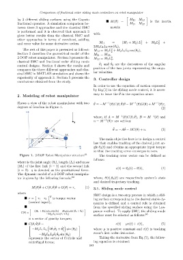
Shows a view of the robot manipulator with two θ = −M −1 (θ)C(θ, θ)θ − M −1 (θ)G(θ) + M −1 (θ)τ,
˙ ˙
¨
degrees of freedom in Figure 1. (2)
˙
where, if A = M −1 (θ)C(θ, θ), B = M −1 (θ) and
u = M −1 (θ)τ are written:

˙
¨
θ = −Aθ − BG(θ) + u. (3)
The main objective here is to design a control
law that enables tracking of the desired joint an-
gle θ d (t) and obtains an appropriate input torque
so that the tracking error converges to zero.
Figure 1. 2-DOF Robot Manipulator structure 63 The tracking error vector can be defined as
follows:
where is the joint angle (θ i ), length (L i ) and mass
(M i ) of the first link (i = 1) and the second link
(i = 2). g is denoted as the gravitational force. e(t) = θ d (t) − θ(t), (4)
The dynamic model of a 2-DOF robot manipula-
tor is given by the following formula: 64 where, θ(t),θ d (t) are respectively system’s state
and desired trajectory tracking.
˙ ˙
¨
M(θ)θ + C(θ, θ)θ + G(θ) = τ, (1) 3.1. Sliding mode control
where
T SMC design is a two-step process in which a slid-
■ τ = τ 1 τ 2 is torque vector ing surface corresponding to the desired stable dy-
(control input); namics is defined and a control rule is obtained
■ from the specified sliding surface using the Lya-

− (M 1 + M 2 ) gL 1 sin (θ 1 ) − M 2 gL 2 sin (θ 1 + θ 2 ) punov method. To apply SMC, the sliding mode
G(θ) =
−M 2 gL 2 sin (θ 1 + θ 2 ) 65
surface must be selected as follows:
is a vector of gravity torques;
˙ ˙
■ C(θ, θ)θ = s(t) = µe(t) + ˙e(t), (5)
" #
˙ ˙
−M 2 L 1 L 2 2θ 1 θ 2 + θ ˙2 sin (θ 2 ) where µ is positive constant and ˙e(t) is tracking
1
˙ ˙
−M 2 L 1 L 2 θ 1 θ 2 sin (θ 2 ) error’s first order derivative.
represents the vector of Coriolis and Taking the derivative from Eq.(5), the follow-
centrifugal forces; ing equation is obtained:
283