Page 31 - IJOCTA-15-3

Using infinitesimal symmetries for determining the first Maxwell time of geometric control problem on SH(2)

′2
L 1 = ω − (E(ψ t ) − E(ψ)) + k (ψ t − ψ)

+k sn(ψ t ) − sn(ψ) ,

′2
L 2 = 1 (E(ψ t ) − E(ψ)) − k (ψ t − ψ)
2
ω(1−k )

+k sn(ψ t ) − sn(ψ) .
We have L 1 = 0 and L 2 = 0. if and
only if both equations,

h 1 = 2k( sn(ψ t ) − sn(ψ) = 0 and
′2
h 2 = (E(ψ t ) − E(ψ)) − k (ψ t − ψ) = 0,
hold. The equation h 1 = 0 holds exclu-
sively when t = 4nkK with k ∈ (0, 1).
Here
R π/2 dt
2
K(k) = √ , k ′2 = 1 − k ,
0 1−k sin t
2
2
for these given values, it follows that
′2
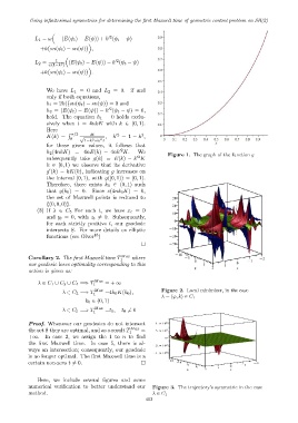
h 2 (4nkK) = 4nE(k) − 4nk K. We Figure 1. The graph of the function g
′2
subsequently take g(k) = E(k) − k K
k ∈ [0, 1) we observe that its derivative
′
g (k) = kK(k), indicating g increases on
the interval [0, 1), with g([0, 1)) = [0, 1).
Therefore, there exists k 0 ∈ (0, 1) such
that g(k 0 ) = 0. Since z(4nk 0 K) = 0,
the set of Maxwell points is reduced to
{(0, 0, 0)}.
(3) If λ ∈ C 5 For each t, we have x t = 0
and y t = 0, with z t ̸= 0. Subsequently,
for each strictly positive t, our geodesic
intersects S. For more details on elliptic
18
functions (see Olver )
□

Corollary 2. The first Maxwell time T Max where
1
our geodesic loses optimality corresponding to this
action is given as:

λ ∈ C 1 ∪ C 3 ∪ C 4 =⇒ T 1 Max = + ∞
λ ∈ C 2 =⇒ T 1 Max =4k 0 K(k 0 ), Figure 2. Local minimizer, in the case
λ = (φ, k) ∈ C 1
k 0 ∈ (0, 1)
λ ∈ C 5 =⇒ T 1 Max =t 0 , t 0 ̸= 0

Proof. Whenever our geodesics do not intersect
the set S they are optimal, and as a result T Max =
1
+∞. In case 2, we assign the 1 to n to find
the first Maxwell time. In case 5, there is al-
ways an intersection; consequently, our geodesic
is no longer optimal. The first Maxwell time is a
certain non-zero t ̸= 0. □

Here, we include several figures and some
numerical verification to better understand our Figure 3. The trajectory’s symmetric in the case
method. λ ∈ C 1
403