Page 49 - IJOCTA-15-3

Modeling and analysis of the dynamics of an excessive gambling problem with modified fractional operator

16
Figure 13 depicts the solutions of N(t) and R(t)
14 obtained by the CF and mABC approaches.
The reader may see from these illustrations
12
P (t) that our model solutions are found to be in
10 good agreement under both fractional opera-
tors. Figure 14 shows the results of A(t) and
8 υ = 0.65 υ = 0.75 υ = 0.85 υ = 0.95
M(t) obtained by the CF and mABC derivatives.
6 100
0 20 40 60 80 100 mABC CF CF mABC
t
80 A(t), ℘ = 0.1
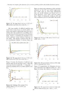
Figure 11. The approximate solutions of P(t) with
Population
different fractional order values when R 0 > 1 60

The large number of addicted gamblers can 40 M(t),ς = 0.005
result from a daily focus on reward values. To
20
reduce this number, individuals must focus on re-
ducing their daily investment in gambling activi-
0
ties and return to their previous non-problematic 0 20 40 60 80 100
t
stage. Figure 11 indicates the dynamics of ad-
dicted gamblers under different fractional or-
Figure 14. Solutions of the system 7 for C-F and
der values. The graph is plotted when the ba-
mABC with υ = 0.70
sic reproduction number is greater than one.
14
υ = 0.95 υ = 0.75 υ = 0.55 υ = 0.35 υ = 0.15
12 140
10
120
P (t) 8 100
6
R(t)
4 80
2 60
0
0 20 40 60 80 100 40
t υ = 0.65 υ = 0.75 υ = 0.85 υ = 0.95
20
Figure 12. The approximate solutions of P(t) with 0
different fractional order values when R 0 < 1 0 20 40 60 80 100
t
Figure 12 shows the behavior of addicted pop-
Figure 15. The approximate solutions of R(t) with
ulation with several fractional order υ when the
different fractional order values
basic reproduction number R 0 < 1. Since R 0 < 1,
gambling problems will not persist (GPFE is sta- Figure 15 demonstrates the dynamics of recov-
ble). ered individuals with different values of υ. Also,
Figure 16 shows the effects of recovery rate ς.
300
R(t) 140
250
mABC
CF 120
200
Population 150 100
80
CF
100
mABC
N(t) R(t) 60
50
40
0 20 ς = 0.0025 ς = 0.005 ς = 0.0075 ς = 0.015
0 20 40 60 80
t 0
0 20 40 60 80 100
t
Figure 13. Solutions of the system (7) for
Caputo–Fabrizio (CF) and mABC with
Figure 16. The approximate solutions of R(t) with
υ = 0.35, α 1 = 1
different values recovery rate ς when υ = 0.75
421