Page 47 - IJOCTA-15-3

Modeling and analysis of the dynamics of an excessive gambling problem with modified fractional operator
5.2. Sensitivity analysis 3

Performing a sensitivity analysis on the gambling 2.5
model helps to identify which model parameters 2
most significantly influence the system’s behav- ℜ 0 1.5
ior. Next, we calculate the normalized sensitivity
index for R 0 with respect to the model parameter 1
p as: 0.5
p ∂R 0
S p = × . 0 0 0.2 0.4 0.6 0.8 1
R 0 ∂p
α 2
The sensitive parameters and their sensitivity in-
dex are shown in Table 2. Figure 3. Effects of a parameter α 2 on the basic
reproduction number R 0
Table 2. Sensitivity indices of R 0
2
Parameter Sensitivity index
α 1 +0.1765
1.5
α 2 +1.0000
γ 2 +1.0000 ℜ 0 1
ψ −0.0200
℘ −0.1681
0.5
λ −0.8140
ς −0.1744 0
+0.1765 0 0.2 0.4 0.6 0.8 1
γ 1
ς
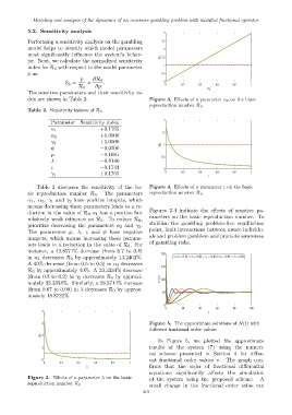
Table 2 discusses the sensitivity of the ba- Figure 4. Effects of a parameter ς on the basic
sic reproduction number R 0 . The parameters reproduction number R 0
α 1 , α 2 , γ 1 and γ 2 have positive imapcts, which
means decreasing these parameters leads to a re-
Figures 2-4 indicate the effects of senstive pa-
duction in the value of R 0 α 1 has a positive but
relatively weak influence on R 0 . To reduce R 0 , rameters on the basic reproduction number. To
prioritize decreasing the parameters α 2 and γ 2 . stabilize the gambling problem-free equilibrium
The parameters ℘, λ, ς and ψ have negative point, limit interactions between aware individu-
imapcts, which means increasing these parame- als and problem gamblers and promote awareness
ters leads to a reduction in the value of R 0 . For of gambling risks.
instance, a 42.8571% decrease (from 0.7 to 0.4)
200
in α 1 decreases R 0 by approximately 13.2402%. υ = 0.10 υ = 0.20 ς = 0.30 υ = 0.40 υ = 0.50
A 40% decrease (from 0.5 to 0.3) in α 2 decreases
150
R 0 by approximately 40%. A 33.3334% decrease
(from 0.3 to 0.2) in γ 2 decreases R 0 by approxi- N (t) 100
mately 33.3334%. Similarly, a 28.5714% increase
(from 0.07 to 0.09) in λ decreases R 0 by approx-
50
imately 18.8722%.
0
0 20 40 60 80 100
8
t
6 Figure 5. The approximate solutions of N(t) with
different fractional order values
4 ℜ 0
In Figure 5, we plotted the approximate
2 results of the system (7) using the numeri-
cal scheme presented in Section 4 for differ-
0 ent fractional order values υ. The graph con-
0 0.2 0.4 0.6 0.8 1
λ firms that the order of fractional differential
equations significantly affects the simulation
Figure 2. Effects of a parameter λ on the basic of the system using the proposed scheme. A
reproduction number R 0
small change in the fractional order value can
419