Page 46 - IJOCTA-15-3

M. Aychluh et.al. / IJOCTA, Vol.15, No.3, pp.407-425 (2025)

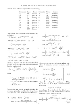
Table 1. Value of the model parameters for equation (7)

Parameter Value Source Parameter Value Source
N 0 200 Assumed A 0 75 Assumed
M 0 42 Assumed P 0 14 Assumed
R 0 0 Assumed Λ 0.33 Calculated
α 1 0.7 10 λ 0.07 10
γ 1 0.2 Assumed ℘ 0.02 Assumed
γ 2 0.3 Assumed ς 0.015 Assumed
γ 3 0.4 Assumed κ 0.34 10
α 2 0.5 Assumed δ 0.014 Assumed
α 3 0.2 Assumed ζ 0.01 Assumed
ψ 0.001 Assumed

The modified fractional-order system with mABC
derivative: γ 1 A + γ 2 M + γ 3 P
+ d A α 1 N + λM + κP
∗ υ γ 1 A+γ 2 M+γ 3 P 
D N(t) = Λ − α 1 N T − ψN  T
t


γ 2 M + γ 3 P


∗ υ γ 1 A+γ 2 M+γ 3 P  − ℘ + α 2 + ψ A

D A(t) = α 1 N + λM + κP 
t T  T





 γ 2 M + γ 3 P

γ 2 M+γ 3 P  A + δP
− ℘ + α 2 + ψ A  + d M α 2
T  T





 γ 3 P


∗ υ γ 2 M+γ 3 P − λ + ς + (1 − c)α 3 + ψ M
D M(t) = α 2 A + δP T
t T



γ 3 P



h i M − (κ + δ + ζ + ψ)P
γ 3 P  + d P (1 − c)α 3

− λ + ς + (1 − c)α 3 + ψ M  T
T 


+ d R [℘A + ςM + ζP − ψR] (33)




∗ υ γ 3 P 
D P(t) = (1 − c)α 3 M − (κ + δ + ζ + ψ)P 

t T 




∗ υ 
D R(t) = ℘A + ςM + ζP − ψR
t
The main objective is to find the optimal control
where d N , d A , d M , d P and d R are adjoint vari-
unit c(t) such that the following control objective
ables. To obtain the necessary optimality condi-
function is minimized:
tions:
Z T 1 
2
J(u) = A 1 M(t) + A 2 P(t) + Bc (t) dt ∗ D Φ i (t) = ∂H (t) 
υ

t
0 2 0 ∂d Φ i 


(32) 




where: ∂H
∗ υ (t) = − (t) (34)
0 D d Φ i
t
∂Φ i 




• A 1 , A 2 > 0: Weights for at-risk and ad- ∂H 


dicted populations. (t) = 0, i = 1, 2, 3, 4, 5. 

∂c
• B > 0: Cost weight for control implemen-
where Φ 1 = N(t), Φ 2 = A(t), Φ 3 = M(t),
tation.
Φ 4 = P(t) and Φ 5 = R(t). The transversality
• T: Final time
conditions:
} .
d i (T) = 0, i ∈ {d Φ i
To solve the new system, we need to derive the
Accordingly, the optimal control c ∗ (t) of a new
necessary optimality conditions for the problem.
dynamic system, which minimizes the objective
To do this, we define the Hamiltonian function:
functional (32), is characterized by
c ∗ (t) =
1 ! !
2
H = A 1 M(t) + A 2 P(t) + Bc (t) γ 3 P(t) M(t)(d P (t) − d M (t))
2 α 3 T
min max 0, , 1 .
γ 1 A + γ 2 M + γ 3 P B
+ d N Λ − α 1 N − ψN
T (35)
418