Page 57 - IJOCTA-15-3

Predefined-time fractional-order terminal SMC for robot dynamics

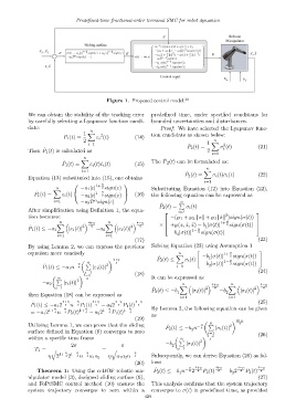
Figure 1. Proposed control model. 32

We can obtain the stability of the tracking error predefined time, under specified conditions for
by carefully selecting a Lyapunov function candi- bounded uncertainties and disturbances.
date: Proof: We have selected the Lyapunov func-
n
1 X tion candidate as shown below:
2
P 1 (t) = ε i (t) (14)
2 n
i=1 P 2 (t) = 1 X σ (t) (21)
2
˙
Then P 1 (t) is calculated as 2 i
i=1
n
˙
X The P 2 (t) can be formulated as:
˙
P 1 (t) = ε i (t) ˙ε i (t) (15)
n
i=1 X
˙
P 2 (t) = σ i (t) ˙σ i (t) (22)
Equation (13) substituted into (15), one obtains
i=1
 1+ η 
n −a 1 |ε| 2 sign(ε) Substituting Equation (12) into Equation (22),
X
˙
P 1 (t) = ε i (t)  −a 2 |ε| 1− η 2 sign(ε)  (16) the following equation can be expressed as
α
i=1 −a 3 D sign(ε) P
n
˙
P 2 (t) = σ i (t)
After simplification using Definition 1, the equa- i=1
2
 
tion becomes: −(℘ 1 + ℘ 2 ∥x∥ + ℘ 3 ∥ ˙x∥ )sign(σ(t))
4+η 4−η  1+ µ 
n
n
X X ×  +℘(x, ˙x, ¨x) − b |σ(t)|
˙ 2 4 2 4 1 2 sign(σ(t)) 
P 1 (t) ≤ −a 1 |ε i (t)| −a 2 |ε i (t)| 1− µ
−b |σ(t)| 2 sign(σ(t))
i=1 i=1 2
(17) (23)
By using Lemma 2, we can express the previous Solving Equation (23) using Assumption 1
equation more concisely n " 1+ µ #
X −b |σ(t)| 2 sign(σ(t))
˙
4+η P 2 (t) ≤ σ i (t) 1 µ
n 4 −b |σ(t)| 1− 2 sign(σ(t))
η
˙
P 1 (t) ≤ −a 1 n − 4 P |ε i (t)| 2 i=1 2
(24)
i=1
4−η (18)

n 4 It can be expressed as
P 2
−a 2 |ε i (t)|
4+µ n 4−µ
n
i=1 ˙ X 2 4 X 2 4
P 2 (t) ≤ −b 1 |σ i (t)| −b 2 |σ i (t)|
then Equation (18) can be expressed as
i=1 i=1
˙
4 − a 2 2
P 1 (t) ≤ −a 1 2 4+η − η 4 P 1 (t) 4+η 4−η 4−η (25)
4 n
4 P 1 (t)
4
η − η 1+ η 1− η 1− η By Lemma 2, the following equation can be given
1+
= −a 1 2 4 n 4 P 1 (t) 4 − a 2 2 4 P 1 (t) 4
as
(19)
n 4+µ
Utilizing Lemma 1, we can prove that the sliding ˙ − µ P 2 4
P 2 (t) ≤ −b n 4 |σ i (t)|
2
surface defined in Equation (6) converges to zero i=1 (26)
within a specific time frame n 4−µ
4
P 2
−b |σ i (t)|
2π π 2
i=1
T 1 = q = q
η 1− η − η − η
1+
η 2 4 2 4 n 4 a 1 a 2 η a 1 a 2 n 4 Subsequently, we can derive Equation (26) as fol-
(20) lows
˙
4 P 2 (t)
4 − b 2
Theorem 1: Using the n-DOF robotic ma- P 2 (t) ≤ −b n − µ 4 2 4+µ 4+µ 4−µ 4−µ
4 P 2 (t)
4
1 2
nipulator model (3), designed sliding surface (6), (27)
and FoPtSMC control method (10) ensures the This analysis confirms that the system trajectory
system trajectory converges to zero within a converges to σ(t) in predefined time, as provided
429