Page 66 - IJOCTA-15-3

M. A. Touat / IJOCTA, Vol.15, No.3, pp.435-448 (2025)
The last part of the block diagram shown is that of the reference model and the already exist-
the learning mechanism; this part modifies the ing basis of the direct FC.
knowledge base with respect to plant parametric The output p (kt)at instant (kt − t) represents
disturbances. The latter modifications are made the correction to be made to the command at in-
on the output membership functions in order to stant in order to reduce the following error e r (kt).
force the closed-loop system to behave like the ref- In other words, we force the FC to produce the
erence model. According to Figure 1, the learning desired command: u (kt − t) + p (kt) necessary to
mechanism consists of following two parts: a fuzzy cancel the tracking error e r (kt). So, the next time
inverse model (FIM) and a knowledge base mod- we encounter the same circumstances, the com-
ifier (KBM). The fuzzy inverse model is based on mand will be the one that will reduce the tracking
the same inference mechanism as the fuzzy con- error.
troller (FC). The inputs of the FIM are as follows:
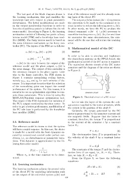
3. Mathematical model of the DC
e r (kt) = y m (kt) − y (kt) (3) motor

In order to be able to simulate and implement
z − 1
c r (kt) = e r (kt) (4) the closed-loop systems on the FPGA board, the
z mathematical model of the DC motor is required.
e r (kt) is the error between the output of the
The equivalent electric circuit of the DC motor
reference model and the plant output; c r (kt) is
armature and the diagram of the rotor are shown
the error change. The output of this controller is
in Figure 3.
the necessary changes in the plant inputs. Like-
R L T
wise to the fuzzy controller, the FIM shown in θ
Figure 1 contains normalizing scaling factors,
namely g em , g cm and g p for each universe of dis- + i +
v e J
course. It is important to notice that the selection
- -
of the normalizing gains can impact the overall
performance of the system. For this reason, it is .
bθ
essential to use an optimization algorithm to com- Armature circuit Rotor
pute these parameters. This is done by using the
MATLAB/Simulink response optimization tool. Figure 3. Electrical circuit of a DC motor
The output of the FIM represents the variation of
Let us take the input of the system the volt-
the FC’s output membership function center. In
age source v applied to the motor armature, while
order to get a better performance, modification of the output is the position of the shaft θ.
the FC rule base is performed by the knowledge
Generally, the torque generated by the DC
base modifier (KBM).
motor is proportional to the armature current and
the magnetic fields. Suppose that the latter is
constant; therefore, the torque T is proportional
2.2. Reference model to the current of the armature i by a constant
factor K 1 :
The reference model is chosen so that the system
will have a rapid response. In this case, the choice
T = K 1 i (6)
is made for a model with the best dynamics en-
sured by conventional control under perfect con- The electromotive force E is proportional to
˙
ditions, i.e., no disturbances or parametric varia- the velocity of the shaft θ by a constant factor
tions. This dynamic is approximated by the fol- K 2 :
lowing first-order model:
E = K 2 θ ˙ (7)
1
R (s) = (5) The constants of the torque T and the electro-
1 + τ m s motive force E are equal, i.e., K 1 = K 2 . There-
Where τ m is the time constant to be deter- fore, we take K 1 = K 2 = K.
mined. From the Figure 3, we have the following
equations:
2.3. Learning mechanism
¨
˙
Jθ + bθ = Ki (8)
The learning mechanism adjusts the ground rules
of the direct FC by exploiting information such di ˙
as the output of the controlled system y (kt) and L + Ri = v − Kθ (9)
dt
438