Page 86 - IJOCTA-15-3

C. D’Apice et .al. / IJOCTA, Vol.15, No.3, pp.449-463 (2025)

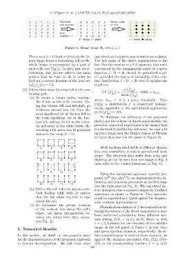
Figure 1. Binary image B j with l j = 1

Then every 2 × 2 block of pixels in the bi- just direct and adaptive segmentation procedures.
nary image forms a contouring cell, so the The key point of the direct segmentation is the
whole image is represented by a grid of fact that the number m+1 of segments that must
such cells (see Fig.1). In fact, just for il- correspond to the homogeneity zones of a given
lustration, this picture reflects the main function f : Ω → R, should be prescribed a pri-
actions that we have to do in order to ori, provided the degree of variability of the orig-
find out a correct location of the level set inal distribution f : Ω → R over Ω satisfies the
φ 0 ε,τ ρ (x) = 1.5. condition
(2) Follow these steps for every cell in the con- σ f

Ω
CV f = · 100% > δ min ,
touring grid: Ω mean f
(a) To create a binary index, combine Ω
where δ min > 0 is a given threshold. Typ-
the 4 bits at the cell’s corners: Us-
ically, a distribution f is considered homoge-
ing the bitwise OR and left-shift, go
neous, especially in the agricultural application,
clockwise around the cell from the
most significant bit at the top left to if CV (f Ω ) ≤ 15%.
the least significant bit at the bot- To illustrate the efficiency of the proposed
tom left, adding the bit to the index. model and the scheme of direct segmentation, we
As indicated in the table below, the provided numerical experiences with images that
resulting 4-bit index has 16 potential the Sentinel-2 satellite has delivered. we used a 10
values in the range 0 − 15. m/pixel image over the Dnipro region of Ukraine
as input data (see the left panel in Figure 3).

0 1 2 3 With medium-sized fields of different shapes,
this area exemplifies a typical agricultural land-
scape. The observed data suffer from noise and
4 5 6 7 blurring, as can be seen from the image in Fig. 3
(also refer to the related histogram in Fig. 4).

8 9 10 11
Using the variational approach recently pro-
posed in 40 (see also 7,8 ), we implemented the de-
blurring and denoizing procedure as the first stage
12 13 14 15
(see the right panel in Fig. 3). The smoothed pic-
(b) Utilize the cell index to access a pre- ture histogram has a marked compactly localized
built lookup table with 16 entries spectrum, as shown in Figure 4. This spectrum
that list the edges required to rep- could be regarded as a “good option”for its piece-
resent the cell. wise constant approximation.
(c) To determine the precise location
Numerical simulations of f-decomposition fol-
of the contour line along the cell’s
lowing the scheme of the direct segmentation have
edges, use linear interpolation be-
been performed considering three different vari-
tween the initial field data values.
ants setting f(x) = u i (x), in Ω, where u i with
(see Fig. 2).
i = 1, 2, 3 stands for the intensity of the satellite
image at the left panel of Figure 1 in red, blue,
5. Numerical Results
and green spectral channels, respectively. To de-
In this section, we dwell on two possible ways fine a segmentation in each of these channels, we
for the implementation of the proposed approach applied the iteration procedure (51), (52), (53)–
to domain decomposition. We call these ways (55) to the corresponding function f = u i with
458