Page 94 - IJOCTA-15-3

Sayed Saber et.al. / IJOCTA, Vol.15, No.3, pp.464-482 (2025)
a 12 , a 13 , and a 14 characterize the effects of β- 2. Stability investigation
cell-derived insulin on lowering glucose levels,
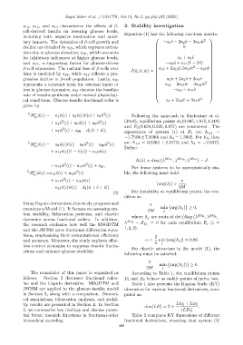
Equation (1) has the following Jacobian matrix:
including both negative modulation and auxil-
 2 
iary impacts. The dynamics of β-cell growth and −a s ˆv − 2a g ˆu − 3a 10 ˆu
decline are detailed by a 15 , which captures activa-  0 
 
tion due to glucose elevation; a 16 , which accounts  
 
for inhibitory influences at higher glucose levels;  −a 1 + a 2 ˆv 
 
and a 17 , a supporting factor for glucose-driven  −a 8 ˆu + a 11 (1 − 2ˆv) 
 2 
β-cell expansion. The natural loss of β-cells over  a 15 + 2a 16 ˆv 3a 17 ˆv − a 19 ˆw 
J(ˆu, ˆv, ˆw) =  
time is modeled by a 18 , while a 19 reflects a pro-  
 
a 2 ˆu + 2a 3 ˆv + 3a 4 ˆv 
gressive decline in β-cell population. Lastly, a 20

 
represents a constant term for external input or  −a 12 − 2a 13 ˆw − 3a 14 ˆw 2 
 
loss in glucose dynamics. a 21 denotes the baseline  −a 18 − a 19 ˆv 
 
rate of insulin synthesis under normal physiologi-  
cal conditions. Glucose-insulin fractional order is a 5 + 2a 6 ˆw + 3a 7 ˆw 2
given by
C α 2
D ˆu(ι) = − a 1 ˆu(ι) + a 2 ˆu(ι)ˆv(ι) + a 3 ˆv (ι) Following the approach in Shabestari et al.
0,ι
2
3
+ a 4 ˆv (ι) + a 5 ˆw(ι) + a 6 ˆw (ι) (2018), equilibrium points E 1 (0.805, 1.815, 1.319)
and E 2 (0.624, 0.935, 0.877) are considered. The
3
+ a 7 ˆw (ι) + a 20 − d 1 (ˆv + ˆw), eigenvalues of system (1) at E 1 are Λ 1,2 =
−1.7564 ± 7.5090i and Λ 3 = 1.3802. For E 2 , they
C α 2 3 are Λ 1,2 = 0.5262 ± 2.3472i and Λ 3 = −2.8372.
D ˆv(ι) = − a 8 ˆu(ι)ˆv(ι) − a 9 ˆu (ι) − a 10 ˆu (ι)
0,ι
Define:
+ a 11 ˆv(ι)(1 − ˆv(ι)) − a 12 ˆw(ι)

∆(λ) = diag λ Mα 1 , λ Mα 2 , λ Mα 3 − J.
2
3
− a 13 ˆw (ι) − a 14 ˆw (ι) + a 21 ,
For linear systems to be asymptotically sta-
C α 2
D w(ι) =a 15 ˆv(ι) + a 16 ˆv (ι) ble, the following must hold:
ˆ
0,ι
3
+ a 17 ˆv (ι) − a 18 ˆw(ι) π
| arg(λ)| > .
− a 19 ˆv(ι) ˆw(ι) − d 2 (ˆu + ˆv + ˆw). 2M
(2) For instability at equilibrium points, the con-
dition is:
Using Caputo derivatives, this study proposes and π
examines a Model (1). It focuses on assessing sys- − min {arg(Λ j )} ≥ 0,
2M j
tem stability, bifurcation patterns, and chaotic
where Λ j are roots of det diag λ Mq x , λ Mq y ,
dynamics across fractional orders. In addition,
λ Mq z − J E j = 0 for each equilibrium E j (i =
the research evaluates how well the MSGDTM
1, 2, 3).
and the JSCSM solve fractional differential equa-
tions, emphasizing their computational efficiency 2
and accuracy. Moreover, the study explores effec- α < min |arg(Λ j )| ≈ 0.86.
π j
tive control strategies to suppress chaotic fluctu-
For chaotic attractors in the model (1), the
ations and enhance glucose stability.
following must be satisfied:
π
− min {|arg(Λ j )|} ≥ 0.
2M j
The remainder of this paper is organized as According to Table 1, the equilibrium points
follows. Section 2 discusses fractional calcu- E 1 and E 2 behave as saddle points of index two.
lus and the Caputo derivative. MSGDTM and Table 1 also presents the Kaplan-Yorke (KY)
JSCSM are applied to the glucose-insulin model dimension for various fractional derivatives, com-
in Section 3, along with a comparison. Numeri- puted as:
cal simulations, bifurcation analyses, and stabil-
ity results are presented in Section 4. In Section LE 1 + LE 2
dim(LE) = 2 + .
5, we summarize key findings and discuss poten- |LE 3 |
tial future research directions in fractional-order Table 2 compares KY dimensions of different
biomedical modeling. fractional derivatives, revealing that system (1)
466