Page 97 - IJOCTA-15-3

Application of Jumarie-Stancu collocation series method and multi-Step
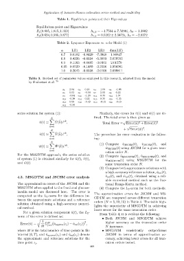
Table 1. Equilibrium points and their Eigenvalues

Equilibrium point and Eigenvalues
E 1 (0.805, 1.815, 1.319) Λ 1,2 = −1.7564 ± 7.5090i, Λ 3 = 1.3802
E 2 (0.624, 0.935, 0.877) Λ 1,2 = 0.5262 ± 2.3472i, Λ 3 = −2.8372

Table 2. Lyapunov Exponents vs. α for Model (1)

α LE1 LE2 LE3 dim(LE)
0.7 0.0182 -0.8429 -7.3948 1.88847
0.8 0.4326 -0.0034 -5.3810 2.079762
0.9 0.1163 -0.0685 -3.0441 2.01570
0.95 0.0529 -0.1489 -2.2316 1.956981
1.0 0.2045 -0.0038 -2.0108 2.099811

Table 3. Revised set of parameter values employed in this research, adapted from the model
by Shabestari et al. 75

a 1 2.04 a 2 0.10 a 3 1.09 a 4 -1.08
a 5 0.03 a 6 -0.06 a 7 2.01 a 8 0.22
a 9 -3.84 a 10 -1.20 a 11 0.30 a 12 1.37
a 13 -0.30 a 14 0.22 a 15 0.30 a 16 -1.35
a 17 0.50 a 18 -0.42 a 19 -0.15 a 20 -0.19
a 21 -0.56

series solution for system (1): Similarly, the errors for ˆv(t) and ˆw(t) are de-
K fined. The total error is then given as:
X
αk
ˆ ˆ
ˆ u(t) ≃ U(k)ι , Total Error = Error(ˆu) + Error(ˆv) 2
p
2
k=0 √ 2
+ Error( ˆw) .
K
X αk
ˆ ˆ
ˆ v(t) ≃ V (k)ι , The procedure for error evaluation is the follow-
k=0 ing:
K
ˆ ˆ
X αk (1) Compute ˆ u JSCSM (t), ˆ v JSCSM (t), and
ˆ w(t) ≃ W(k)ι .
ˆ w JSCSM (t) using JSCSM for a given trun-
k=0
cation order N.
For the MSGDTM approach, the series solution
(2) Compute ˆu MSGDTM (t), ˆv MSGDTM (t), and
of system (1) is obtained similarly for ˆu(t), ˆv(t),
ˆ w MSGDTM (t) using MSGDTM for the
and ˆw(t).
same truncation order N.
(3) Compare both approximate solutions with
a high-accuracy reference solution, ˆu ref (t),
4.3. MSGDTM and JSCSM error analysis ˆ v ref (t), and ˆw ref (t), obtained using a reli-
able numerical method such as the frac-
The approximation errors of the JSCSM and the tional Runge-Kutta method.
MSGDTM when applied to the fractional glucose- (4) Compute the L 2 -norm for both methods.
insulin model are discussed here. The error is
The approximation errors for JSCSM and MS-
computed as the L 2 -norm for the difference be-
GDTM are compared across different truncation
tween the approximate solutions and a reference orders (N = 5, 10, 15) in Table 4. The table high-
solution obtained using a high-accuracy numeri- lights the superiority of MSGDTM in achieving
cal method.
lower errors for the same truncation order.
For a given solution component ˆu(t), the L 2 -
From Table 4, it is evident the following:
norm of the error is defined as:
• Both JSCSM and MSGDTM achieve
r
1 2 higher accuracy as the truncation order
Error(ˆu) = Σ M ˆ u approx (ι j ) − ˆu ref (ι j ) ,
j=1
M N increases.
where M is the total number of time points in the • MSGDTM consistently outperforms
interval [0, T], and ˆu approx (ι j ) and ˆu ref (ι j ) denote JSCSM in terms of approximation ac-
the approximate and reference solutions for the curacy, achieving lower errors for all trun-
time point ι j . cation orders tested.
469